Macroeconomics

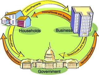
Macroeconomics (from the Greek prefix makro- meaning "large" + economics) is a branch of economics dealing with the performance, structure, behavior, and decision-making of an economy as a whole. This includes regional, national, and global economies.[1][2] Macroeconomists study topics such as GDP, unemployment rates, national income, price indices, output, consumption, unemployment, inflation, saving, investment, energy, international trade, and international finance.

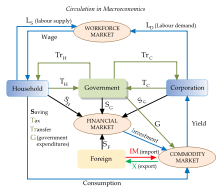
Macroeconomics takes a big-picture view of the entire economy, including examining the roles of, and relationships between, corporations, governments and households, and the different types of markets, such as the financial market and the labour market.

Macroeconomics and microeconomics are the two most general fields in economics.[3]

Development

Main article: History of macroeconomic thought

Origins

Macroeconomics descended from the once divided fields of business cycle theory and monetary theory.[4] The quantity theory of money was particularly influential prior to World War II. It took many forms, including the version based on the work of Irving Fisher:

${\displaystyle M\cdot V=P\cdot Q}$

In the typical view of the quantity theory, money velocity (V) and the quantity of goods produced (Q) would be constant, so any increase in money supply (M) would lead to a direct increase in price level (P). The quantity theory of money was a central part of the classical theory of the economy that prevailed in the early twentieth century.

Austrian School

Ludwig Von Mises's work Theory of Money and Credit, published in 1912, was one of the first books from the Austrian School to deal with macroeconomic topics.

Keynes and his followers

Macroeconomics, at least in its modern form,[5] began with the publication of John Maynard Keynes's General Theory of Employment, Interest and Money.[4][6] When the Great Depression struck, classical economists had difficulty explaining how goods could go unsold and workers could be left unemployed. In classical theory, prices and wages would drop until the market cleared, and all goods and labor were sold. Keynes offered a new theory of economics that explained why markets might not clear, which would evolve (later in the 20th century) into a group of macroeconomic schools of thought known as Keynesian economics – also called Keynesianism or Keynesian theory.

In Keynes's theory, the quantity theory broke down because people and businesses tend to hold on to their cash in tough economic times – a phenomenon he described in terms of liquidity preferences. Keynes also explained how the multiplier effect would magnify a small decrease in consumption or investment and cause declines throughout the economy. Keynes also noted the role uncertainty and animal spirits can play in the economy.[5]

The generation following Keynes combined the macroeconomics of the General Theory with neoclassical microeconomics to create the neoclassical synthesis. By the 1950s, most economists had accepted the synthesis view of the macroeconomy.[5] Economists like Paul Samuelson, Franco Modigliani, James Tobin, and Robert Solow developed formal Keynesian models and contributed formal theories of consumption, investment, and money demand that fleshed out the Keynesian framework.[7]

Monetarism

Milton Friedman updated the quantity theory of money to include a role for money demand. He argued that the role of money in the economy was sufficient to explain the Great Depression, and that aggregate demand oriented explanations were not necessary. Friedman also argued that monetary policy was more effective than fiscal policy; however, Friedman doubted the government's ability to "fine-tune" the economy with monetary policy. He generally favored a policy of steady growth in money supply instead of frequent intervention.[8]

Friedman also challenged the Phillips curve relationship between inflation and unemployment. Friedman and Edmund Phelps (who was not a monetarist) proposed an "augmented" version of the Phillips curve that excluded the possibility of a stable, long-run tradeoff between inflation and unemployment.[9] When the oil shocks of the 1970s created a high unemployment and high inflation, Friedman and Phelps were vindicated. Monetarism was particularly influential in the early 1980s. Monetarism fell out of favor when central banks found it difficult to target money supply instead of interest rates as monetarists recommended. Monetarism also became politically unpopular when the central banks created recessions in order to slow inflation.

New classical

New classical macroeconomics further challenged the Keynesian school. A central development in new classical thought came when Robert Lucas introduced rational expectations to macroeconomics. Prior to Lucas, economists had generally used adaptive expectations where agents were assumed to look at the recent past to make expectations about the future. Under rational expectations, agents are assumed to be more sophisticated. A consumer will not simply assume a 2% inflation rate just because that has been the average the past few years; they will look at current monetary policy and economic conditions to make an informed forecast. When new classical economists introduced rational expectations into their models, they showed that monetary policy could only have a limited impact.

Lucas also made an influential critique of Keynesian empirical models. He argued that forecasting models based on empirical relationships would keep producing the same predictions even as the underlying model generating the data changed. He advocated models based on fundamental economic theory that would, in principle, be structurally accurate as economies changed. Following Lucas's critique, new classical economists, led by Edward C. Prescott and Finn E. Kydland, created real business cycle (RB C) models of the macro economy.[10]

RB C models were created by combining fundamental equations from neo-classical microeconomics. In order to generate macroeconomic fluctuations, RB C models explained recessions and unemployment with changes in technology instead of changes in the markets for goods or money. Critics of RB C models argue that money clearly plays an important role in the economy, and the idea that technological regress can explain recent recessions is implausible.[10] However, technological shocks are only the more prominent of a myriad of possible shocks to the system that can be modeled. Despite questions about the theory behind RB C models, they have clearly been influential in economic methodology.[11]

New Keynesian response

New Keynesian economists responded to the new classical school by adopting rational expectations and focusing on developing micro-founded models that are immune to the Lucas critique. Stanley Fischer and John B. Taylor produced early work in this area by showing that monetary policy could be effective even in models with rational expectations when contracts locked in wages for workers. Other new Keynesian economists, including Olivier Blanchard, Julio Rotemberg, Greg Mankiw, David Romer, and Michael Woodford, expanded on this work and demonstrated other cases where inflexible prices and wages led to monetary and fiscal policy having real effects.

Like classical models, new classical models had assumed that prices would be able to adjust perfectly and monetary policy would only lead to price changes. New Keynesian models investigated sources of sticky prices and wages due to imperfect competition,[12] which would not adjust, allowing monetary policy to impact quantities instead of prices.

By the late 1990s economists had reached a rough consensus. The nominal rigidity of new Keynesian theory was combined with rational expectations and the RBC methodology to produce dynamic stochastic general equilibrium (DSGE) models. The fusion of elements from different schools of thought has been dubbed the new neoclassical synthesis. These models are now used by many central banks and are a core part of contemporary macroeconomics.[13]

New Keynesian economics, which developed partly in response to new classical economics, strives to provide microeconomic foundations to Keynesian economics by showing how imperfect markets can justify demand management.

Macroeconomic models

Aggregate demand–aggregate supply

A traditional AS–AD diagram showing a shift in AD and the AS curve becoming inelastic beyond potential output.

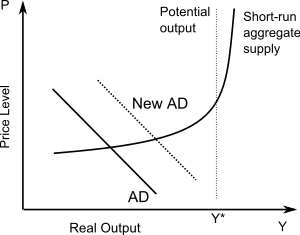
The AD-AS model has become the standard textbook model for explaining the macroeconomy.[14] This model shows the price level and level of real output given the equilibrium in aggregate demand and aggregate supply. The aggregate demand curve's downward slope means that more output is demanded at lower price levels.[15] The downward slope is the result of three effects: the Pigou or real balance effect, which states that as real prices fall, real wealth increases, resulting in higher consumer demand of goods; the Keynes or interest rate effect, which states that as prices fall, the demand for money decreases, causing interest rates to decline and borrowing for investment and consumption to increase; and the net export effect, which states that as prices rise, domestic goods become comparatively more expensive to foreign consumers, leading to a decline in exports.[15]

In the conventional Keynesian use of the AS-AD model, the aggregate supply curve is horizontal at low levels of output and becomes inelastic near the point of potential output, which corresponds with full employment.[14] Since the economy cannot produce beyond the potential output, any AD expansion will lead to higher price levels instead of higher output.

The AD–AS diagram can model a variety of macroeconomic phenomena, including inflation. Changes in the non-price level factors or determinants cause changes in aggregate demand and shifts of the entire aggregate demand (AD) curve. When demand for goods exceeds supply there is an inflationary gap where demand-pull inflation occurs and the AD curve shifts upward to a higher price level. When the economy faces higher costs, cost-push inflation occurs and the AS curve shifts upward to higher price levels.[16] The AS–AD diagram is also widely used as a pedagogical tool to model the effects of various macroeconomic policies.[17]

IS-LM

In this example of an IS/LM chart, the IS curve moves to the right, causing higher interest rates (i) and expansion in the "real" economy (real GDP, or Y).

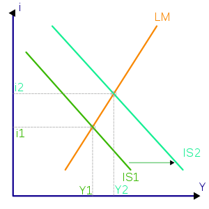
The IS–LM model gives the underpinnings of aggregate demand (itself discussed above). It answers the question "At any given price level, what is the quantity of goods demanded?" This model shows what combination of interest rates and output will ensure equilibrium in both the goods and money markets.[18] The goods market is modeled as giving equality between investment and public and private saving (IS), and the money market is modeled as giving equilibrium between the money supply and liquidity preference.[19]

The IS curve consists of the points (combinations of income and interest rate) where investment, given the interest rate, is equal to public and private saving, given output[20] The IS curve is downward sloping because output and the interest rate have an inverse relationship in the goods market: as output increases, more income is saved, which means interest rates must be lower to spur enough investment to match saving.[20]

The LM curve is upward sloping because the interest rate and output have a positive relationship in the money market: as income (identically equal to output) increases, the demand for money increases, resulting in a rise in the interest rate in order to just offset the incipient rise in money demand.[21]

The IS-LM model is often used to demonstrate the effects of monetary and fiscal policy.[18] Textbooks frequently use the IS-LM model, but it does not feature the complexities of most modern macroeconomic models.[18] Nevertheless, these models still feature similar relationships to those in IS-LM.[18]

Growth models

The neoclassical growth model of Robert Solow has become a common textbook model for explaining economic growth in the long-run. The model begins with a production function where national output is the product of two inputs: capital and labor. The Solow model assumes that labor and capital are used at constant rates without the fluctuations in unemployment and capital utilization commonly seen in business cycles.[22]

An increase in output, or economic growth, can only occur because of an increase in the capital stock, a larger population, or technological advancements that lead to higher productivity (total factor productivity). An increase in the savings rate leads to a temporary increase as the economy creates more capital, which adds to output. However, eventually the depreciation rate will limit the expansion of capital: savings will be used up replacing depreciated capital, and no savings will remain to pay for an additional expansion in capital. Solow's model suggests that economic growth in terms of output per capita depends solely on technological advances that enhance productivity.[23]

In the 1980s and 1990s endogenous growth theory arose to challenge neoclassical growth theory. This group of models explains economic growth through other factors, such as increasing returns to scale for capital and learning-by-doing, that are endogenously determined instead of the exogenous technological improvement used to explain growth in Solow's model.[24]

Basic macroeconomic concepts

Macroeconomics encompasses a variety of concepts and variables, but there are three central topics for macroeconomic research.[25] Macroeconomic theories usually relate the phenomena of output, unemployment, and inflation. Outside of macroeconomic theory, these topics are also important to all economic agents including workers, consumers, and producers.

Circulation in macroeconomics.

Output and income

National output is the total amount of everything a country produces in a given period of time. Everything that is produced and sold generates an equal amount of income. The total output of the economy is measured GDP per person. The output and income are usually considered equivalent and the two terms are often used interchangeably, output changes into income. Output can be measured or it can be viewed from the production side and measured as the total value of final goods and services or the sum of all value added in the economy.[26]

Macroeconomic output is usually measured by gross domestic product (GDP) or one of the other national accounts. Economists interested in long-run increases in output study economic growth. Advances in technology, accumulation of machinery and other capital, and better education and human capital are all factors that lead to increase economic output over time. However, output does not always increase consistently over time. Business cycles can cause short-term drops in output called recessions. Economists look for macroeconomic policies that prevent economies from slipping into recessions and that lead to faster long-term growth.

Unemployment

Main article: Unemployment

A chart using US data showing the relationship between economic growth and unemployment expressed by Okun's law. The relationship demonstrates cyclical unemployment. Economic growth leads to a lower unemployment rate.

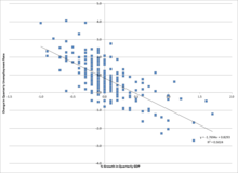
The amount of unemployment in an economy is measured by the unemployment rate, i.e. the percentage of workers without jobs in the labor force. The unemployment rate in the labor force only includes workers actively looking for jobs. People who are retired, pursuing education, or discouraged from seeking work by a lack of job prospects are excluded.

Unemployment can be generally broken down into several types that are related to different causes.

• Classical unemployment theory suggests that unemployment occurs when wages are too high for employers to be willing to hire more workers. Other more modern economic theories suggest that increased wages actually decrease unemployment by creating more consumer demand. According to these more recent theories, unemployment results from reduced demand for the goods and services produced through labor and suggest that only in markets where profit margins are very low, and in which the market will not bear a price increase of product or service, will higher wages result in unemployment.
• Consistent with classical unemployment theory, frictional unemployment occurs when appropriate job vacancies exist for a worker, but the length of time needed to search for and find the job leads to a period of unemployment.[27]
• Structural unemployment covers a variety of possible causes of unemployment including a mismatch between workers' skills and the skills required for open jobs.[28] Large amounts of structural unemployment commonly occur when an economy shifts to focus on new industries and workers find their previous set of skills are no longer in demand. Structural unemployment is similar to frictional unemployment as both reflect the problem of matching workers with job vacancies, but structural unemployment also covers the time needed to acquire new skills in addition to the short-term search process.[29]
• While some types of unemployment may occur regardless of the condition of the economy, cyclical unemployment occurs when growth stagnates. Okun's law represents the empirical relationship between unemployment and economic growth.[30] The original version of Okun's law states that a 3% increase in output would lead to a 1% decrease in unemployment.[31]

Inflation and deflation

The ten-year moving averages of changes in price level and growth in money supply (using the measure of M2, the supply of hard currency and money held in most types of bank accounts) in the US from 1875 to 2011. Over the long run, the two series show a close relationship.

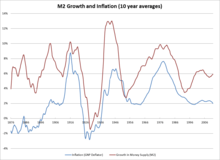
A general price increase across the entire economy is called inflation. When prices decrease, there is deflation. Economists measure these changes in prices with price indexes. Inflation can occur when an economy becomes overheated and grows too quickly. Similarly, a declining economy can lead to deflation.

Central bankers, who manage a country's money supply, try to avoid changes in price level by using monetary policy. Raising interest rates or reducing the supply of money in an economy will reduce inflation. Inflation can lead to increased uncertainty and other negative consequences. Deflation can lower economic output. Central bankers try to stabilize prices to protect economies from the negative consequences of price changes.

Changes in price level may be the result of several factors. The quantity theory of money holds that changes in price level are directly related to changes in the money supply. Most economists believe that this relationship explains long-run changes in the price level.[32] Short-run fluctuations may also be related to monetary factors, but changes in aggregate demand and aggregate supply can also influence price level. For example, a decrease in demand due to a recession can lead to lower price levels and deflation. A negative supply shock, such as an oil crisis, lowers aggregate supply and can cause inflation.

Macroeconomic policy

Macroeconomic policy is usually implemented through two sets of tools: fiscal and monetary policy. Both forms of policy are used to stabilize the economy, which can mean boosting the economy to the level of GDP consistent with full employment.[33] Macroeconomic policy focuses on limiting the effects of the business cycle to achieve the economic goals of price stability, full employment, and growth.[34]

Monetary policy

Further information: Monetary policy

Central banks implement monetary policy by controlling the money supply through several mechanisms. Typically, central banks take action by issuing money to buy bonds (or other assets), which boosts the supply of money and lowers interest rates, or, in the case of contractionary monetary policy, banks sell bonds and take money out of circulation. Usually policy is not implemented by directly targeting the supply of money.

Central banks continuously shift the money supply to maintain a targeted fixed interest rate. Some of them allow the interest rate to fluctuate and focus on targeting inflation rates instead. Central banks generally try to achieve high output without letting loose monetary policy that create large amounts of inflation.

Conventional monetary policy can be ineffective in situations such as a liquidity trap. When interest rates and inflation are near zero, the central bank cannot loosen monetary policy through conventional means.

An example of intervention strategy under different conditions

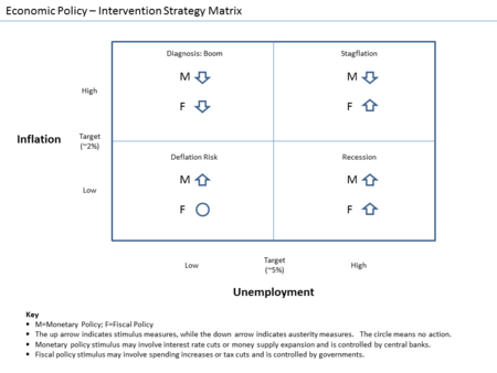
Central banks can use unconventional monetary policy such as quantitative easing to help increase output. Instead of buying government bonds, central banks can implement quantitative easing by buying not only government bonds, but also other assets such as corporate bonds, stocks, and other securities. This allows lower interest rates for a broader class of assets beyond government bonds. In another example of unconventional monetary policy, the United States Federal Reserve recently made an attempt at such a policy with Operation Twist. Unable to lower current interest rates, the Federal Reserve lowered long-term interest rates by buying long-term bonds and selling short-term bonds to create a flat yield curve.

Fiscal policy

Further information: Fiscal policy

Fiscal policy is the use of government's revenue and expenditure as instruments to influence the economy. Examples of such tools are expenditure, taxes, debt.

For example, if the economy is producing less than potential output, government spending can be used to employ idle resources and boost output. Government spending does not have to make up for the entire output gap. There is a multiplier effect that boosts the impact of government spending. For instance, when the government pays for a bridge, the project not only adds the value of the bridge to output, but also allows the bridge workers to increase their consumption and investment, which helps to close the output gap.

The effects of fiscal policy can be limited by crowding out. When the government takes on spending projects, it limits the amount of resources available for the private sector to use. Crowding out occurs when government spending simply replaces private sector output instead of adding additional output to the economy. Crowding out also occurs when government spending raises interest rates, which limits investment. Defenders of fiscal stimulus argue that crowding out is not a concern when the economy is depressed, plenty of resources are left idle, and interest rates are low.[35][36]

Fiscal policy can be implemented through automatic stabilizers. Automatic stabilizers do not suffer from the policy lags of discretionary fiscal policy. Automatic stabilizers use conventional fiscal mechanisms but take effect as soon as the economy takes a downturn: spending on unemployment benefits automatically increases when unemployment rises and, in a progressive income tax system, the effective tax rate automatically falls when incomes decline.

Comparison

Economists usually favor monetary over fiscal policy because it has two major advantages. First, monetary policy is generally implemented by independent central banks instead of the political institutions that control fiscal policy. Independent central banks are less likely to make decisions based on political motives.[33] Second, monetary policy suffers shorter inside lags and outside lags than fiscal policy. Central banks can quickly make and implement decisions while the discretionary fiscal policy may take time to pass and even longer to carry out.[33]

See also

• Dynamic stochastic general equilibrium
• Economic development

Notes

1. O'Sullivan, Arthur; Sheffrin, Steven M. (2003), Economics: Principles in Action, Upper Saddle River, New Jersey 07458: Pearson Prentice Hall, p. 57, ISBN 978-0-13-063085-8CS1 maint: location (link)
2. Steve Williamson, Notes on Macroeconomic Theory, 1999
3. Blaug, Mark (1985), Economic theory in retrospect, Cambridge: Cambridge University Press, ISBN 978-0-521-31644-6
4. Dimand (2008).
5. Blanchard (2011), 580.
6. Snowdon, Brian; Vane, Howard R. (2005). Modern Macroeconomics – Its origins, development and current state. Edward Elgar. ISBN 1-84542-208-2.
7. Blanchard (2011), 581.
8. Blanchard (2011), 582–83.
9. "Phillips Curve: The Concise Encyclopedia of Economics | Library of Economics and Liberty". www.econlib.org. Retrieved 2018-01-23.
10. Blanchard (2011), 587.
11. Kariappa Bheemaiah, The Blockchain Alternative: Rethinking Macroeconomic Policy and Economic Theory (Dordrecht NL: Apress/Springer Nature, 2017), 169-70. ISBN 1484226747, 9781484226742
12. The role of imperfect competition in new Keynesian economics, Chapter 4 of Surfing Economics by Huw Dixon
13. Blanchard (2011), 590.
14. Healey 2002, p. 12.
15. Healey 2002, p. 13.
16. Healey 2002, p. 14.
17. Colander 1995, p. 173. sfn error: no target: CITEREFColander1995 (help)
18. Durlauf & Hester 2008.
19. Peston 2002, pp. 386–87.
20. Peston 2002, p. 387.
21. Peston 2002, pp. 387–88.
22. Solow 2002, pp. 518–19.
23. Solow 2002, p. 519.
24. Blaug 2002, pp. 202–03.
25. Blanchard (2011), 32.
26. Blanchard (2011), 22.
27. Dwivedi, 443.
28. Freeman (2008). http://www.dictionaryofeconomics.com/article?id=pde2008_S000311.
29. Dwivedi, 444–45.
30. Dwivedi, 445–46.
31. Neely, Christopher J. "Okun's Law: Output and Unemployment. Economic Synopses. Number 4. 2010. http://research.stlouisfed.org/publications/es/10/ES1004.pdf.
32. Mankiw 2014, p. 634.
33. Mayer, 495.
34. "AP Macroeconomics Review".
35. Ye, Fred Y. (2017). Scientific Metrics: Towards Analytical and Quantitative Sciences. Springer. ISBN 978-981-10-5936-0.
36. Arestis, Philip; Sawyer, Malcolm (2003). "Reinventing fiscal policy" (PDF). Levy Economics Institute of Bard College (Working Paper, No. 381). Retrieved 7 December 2018.

References

• Blanchard, Olivier (2000). Macroeconomics. Prentice Hall. ISBN 978-0-13-013306-9.CS1 maint: ref=harv (link)
• Blanchard, Olivier (2011). Macroeconomics Updated (5th ed.). Englewood Cliffs: Prentice Hall. ISBN 978-0-13-215986-9.CS1 maint: ref=harv (link)
• Blaug, Mark (1986), Great Economists before Keynes, Brighton: Wheatsheaf.
• Blaug, Mark (2002). "Endogenous growth theory". In Snowdon, Brian; Vane, Howard (eds.). An Encyclopedia of Macroeconomics. Northampton, Massachusetts: Edward Elgar Publishing. ISBN 978-1-84542-180-9.CS1 maint: ref=harv (link)
• Boettke, Peter (2001). Calculation and Coordination: Essays on Socialism and Transitional Political Economy. Routledge. ISBN 978-0-415-77109-2.
• Bouman, John: Principles of Macroeconomics – free fully comprehensive Principles of Microeconomics and Macroeconomics texts. Columbia, Maryland, 2011
• Dimand, Robert W. (2008). Durlauf, Steven N.; Blume, Lawrence E. (eds.). Macroeconomics, origins and history of. The New Palgrave Dictionary of Economics. pp. 236–44. doi:10.1057/9780230226203.1009. ISBN 978-0-333-78676-5.
• Durlauf, Steven N.; Hester, Donald D. (2008). "IS–LM". In Durlauf, Steven N.; Blume, Lawrence E. (eds.). The New Palgrave Dictionary of Economics (2nd ed.). Palgrave Macmillan. pp. 585–91. doi:10.1057/9780230226203.0855. ISBN 978-0-333-78676-5. Retrieved 5 June 2012.CS1 maint: ref=harv (link)
• Dwivedi, D.N. (2001). Macroeconomics: theory and policy. New Delhi: Tata McGraw-Hill. ISBN 978-0-07-058841-7.CS1 maint: ref=harv (link)
• Friedman, Milton (1953). Essays in Positive Economics. London: University of Chicago Press. ISBN 978-0-226-26403-5.
• Haberler, Gottfried (1937). Prosperity and depression. League of Nations.
• Leijonhufvud, Axel The Wicksell Connection: Variation on a Theme. UCLA. November, 1979.
• Healey, Nigel M. (2002). "AD-AS model". In Snowdon, Brian; Vane, Howard (eds.). An Encyclopedia of Macroeconomics. Northampton, Massachusetts: Edward Elgar Publishing. pp. 11–18. ISBN 978-1-84542-180-9.CS1 maint: ref=harv (link)
• Heijdra, Ben J.; van der Ploeg, Frederick (2002). Foundations of Modern Macroeconomics. Oxford University Press. ISBN 978-0-19-877617-8.
• Mankiw, N. Gregory (2014). Principles of Economics. Cengage Learning. ISBN 978-1-305-15604-3.CS1 maint: ref=harv (link)
• Mises, Ludwig Von (1912). Theory of Money and Credit. Yale University Press.
• Mayer, Thomas (2002). "Monetary policy: role of". In Snowdon, Brian; Vane, Howard R. (eds.). An Encyclopedia of Macroeconomics. Northampton, Massachusetts: Edward Elgar Publishing. pp. 495–99. ISBN 978-1-84542-180-9.CS1 maint: ref=harv (link)
• Mishkin, Frederic S. (2004). The Economics of Money, Banking, and Financial Markets. Boston: Addison-Wesley. p. 517.
• Peston, Maurice (2002). "IS-LM model: closed economy". In Snowdon, Brian; Vane, Howard R. (eds.). An Encyclopedia of Macroeconomics. Edward Elgar.CS1 maint: ref=harv (link)
• Reed, Jacob (2016). AP Economics Review, Macroeconomics.
• Solow, Robert (2002). "Neoclassical growth model". In Snowdon, Brian; Vane, Howard (eds.). An Encyclopedia of Macroeconomics. Northampton, Massachusetts: Edward Elgar Publishing. ISBN 1840643870.CS1 maint: ref=harv (link)
• Snowdon, Brian, and Howard R. Vane, ed. (2002). An Encyclopedia of Macroeconomics, Description & scroll to Contents-preview links.
• Snowdon, Brian; Vane, Howard R. (2005). Modern Macroeconomics: Its Origins, Development And Current State. Edward Elgar Publishing. ISBN 1845421809.CS1 maint: ref=harv (link)
• Gärtner, Manfred (2006). Macroeconomics. Pearson Education Limited. ISBN 978-0-273-70460-7.CS1 maint: ref=harv (link)
• Warsh, David (2006). Knowledge and the Wealth of Nations. Norton. ISBN 978-0-393-05996-0.CS1 maint: ref=harv (link)
• Levi, Maurice (2014). The Macroeconomic Environment of Business (Core Concepts and Curious Connections). New Jersey: World Scientific Publishing. ISBN 978-981-4304-34-4.CS1 maint: ref=harv (link)