Consumer choice
The theory of consumer choice is the branch of microeconomics that relates preferences to consumption expenditures and to consumer demand curves. It analyzes how consumers maximize the desirability of their consumption as measured by their preferences subject to limitations on their expenditures, by maximizing utility subject to a consumer budget constraint.[1]
| Part of a series on |
| Economics |
|---|
|
|
|
By application |
|
Notable economists |
|
Lists |
|
Glossary |
|
Consumption is separated from production, logically, because two different economic agents are involved. In the first case consumption is by the primary individual; in the second case, a producer might make something that he would not consume himself. Therefore, different motivations and abilities are involved. The models that make up consumer theory are used to represent prospectively observable demand patterns for an individual buyer on the hypothesis of constrained optimization. Prominent variables used to explain the rate at which the good is purchased (demanded) are the price per unit of that good, prices of related goods, and wealth of the consumer.
The law of demand states that the rate of consumption falls as the price of the good rises, even when the consumer is monetarily compensated for the effect of the higher price; this is called the substitution effect. As the price of a good rises, consumers will substitute away from that good, choosing more of other alternatives. If no compensation for the price rise occurs, as is usual, then the decline in overall purchasing power due to the price rise leads, for most goods, to a further decline in the quantity demanded; this is called the income effect.
In addition, as the wealth of the individual rises, demand for most products increases, shifting the demand curve higher at all possible prices.
The basic problem of consumer theory takes the following inputs:
- The consumption set C – the set of all bundles that the consumer could conceivably consume.
- A preference relation over the bundles of C. This preference relation can be described as an ordinal utility function, describing the utility that the consumer derives from each bundle.
- A price system, which is a function assigning a price to each bundle.
- An initial endowment, which is a bundle from C that the consumer initially holds. The consumer can sell all or some of his initial bundle in the given prices, and can buy another bundle in the given prices. He has to decide which bundle to buy, under the given prices and budget, in order to maximize his utility.
Example: homogeneous divisible goods
Consider an economy with two types of homogeneous divisible goods, traditionally called X and Y.
- The consumption set is , i.e. the set of all pairs where and . Each bundle contains a non-negative quantity of good X and a non-negative quantity of good Y.
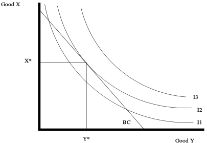
- A typical preference relation in this universe can be represented by a set of indifference curves. Each curve represents a set of bundles that give the consumer the same utility. A typical utility function is the Cobb–Douglas function: , whose indifference curves look like in the figure below.
- A typical price system assigns a price to each type of good, such that the cost of bundle is .
- A typical initial endowment is just a fixed income, which along with the prices implies a budget constraint. The consumer can choose any point on or below the budget constraint line BC In the diagram. This line is downward sloped and linear since it represents the boundary of the inequality . In other words, the amount spent on both goods together is less than or equal to the income of the consumer.
The consumer will choose the indifference curve with the highest utility that is attainable within his budget constraint. Every point on indifference curve I3 is outside his budget constraint so the best that he can do is the single point on I2 where the latter is tangent to his budget constraint. He will purchase X* of good X and Y* of good Y.
Indifference curve analysis begins with the utility function. The utility function is treated as an index of utility.[2] All that is necessary is that the utility index change as more preferred bundles are consumed.
Indifference curves are typically numbered with the number increasing as more preferred bundles are consumed. The numbers have no cardinal significance; for example if three indifference curves are labeled 1, 4, and 16 respectively that means nothing more than the bundles "on" indifference curve 4 are more preferred than the bundles "on" indifference curve 1.
Income effect and price effect deal with how the change in price of a commodity changes the consumption of the good. The theory of consumer choice examines the trade-offs and decisions people make in their role as consumers as prices and their income changes.
Example: land
As a second example, consider an economy which consists of a large land-estate L.
- The consumption set is , i.e. the set of all subsets of L (all land parcels).
- A typical preference relation in this universe can be represented by a utility function which assigns, to each land parcel, its total "fertility" (the total amount of grain that can be grown in that land).
- A typical price system assigns a price to each land parcel, based on its area.
- A typical initial endowment is either a fixed income, or an initial parcel which the consumer can sell and buy another parcel.[3]
Effect of a price change
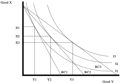
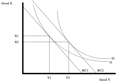
The indifference curves and budget constraint can be used to predict the effect of changes to the budget constraint. The graph below shows the effect of a price increase for good Y. If the price of Y increases, the budget constraint will pivot from BC2 to BC1. Notice that because the price of X does not change, the consumer can still buy the same amount of X if he or she chooses to buy only good X. On the other hand, if the consumer chooses to buy only good Y, he or she will be able to buy less of good Y because its price has increased.
To maximize the utility with the reduced budget constraint, BC1, the consumer will re-allocate consumption to reach the highest available indifference curve which BC1 is tangent to. As shown on the diagram below, that curve is I1, and therefore the amount of good Y bought will shift from Y2 to Y1, and the amount of good X bought to shift from X2 to X1. The opposite effect will occur if the price of Y decreases causing the shift from BC2 to BC3, and I2 to I3.
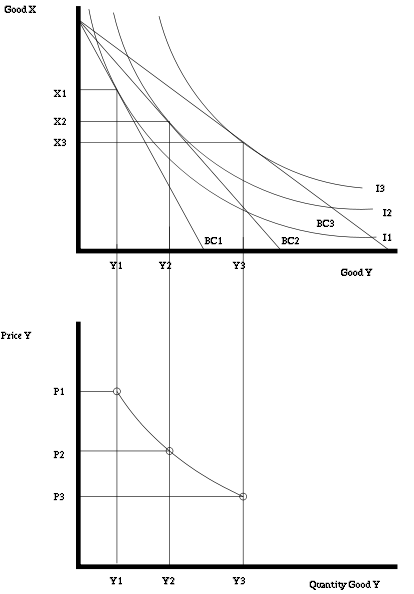
If these curves are plotted for many different prices of good Y, a demand curve for good Y can be constructed. The diagram below shows the demand curve for good Y as its price varies. Alternatively, if the price for good Y is fixed and the price for good X is varied, a demand curve for good X can be constructed.
Income effect
Another important item that can change is the money income of the consumer. The income effect is the phenomenon observed through changes in purchasing power. It reveals the change in quantity demanded brought by a change in real income. Graphically, as long as the prices remain constant, changing income will create a parallel shift of the budget constraint. Increasing the income will shift the budget constraint right since more of both can be bought, and decreasing income will shift it left.
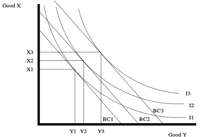
Depending on the indifference curves, as income increases, the amount purchased of a good can either increase, decrease or stay the same. In the diagram below, good Y is a normal good since the amount purchased increased as the budget constraint shifted from BC1 to the higher income BC2. Good X is an inferior good since the amount bought decreased as the income increases.
is the change in the demand for good 1 when we change income from to , holding the price of good 1 fixed at :
Price effect as sum of substitution and income effects
Every price change can be decomposed into an income effect and a substitution effect; the price effect is the sum of substitution and income effects.
The substitution effect is the change in demands resulting from a price change that alters the slope of the budget constraint but leaves the consumer on the same indifference curve. In other words, it illustrates the consumer's new consumption basket after the price change while being compensated as to allow the consumer to be as happy as he or she was previously. By this effect, the consumer is posited to substitute toward the good that becomes comparatively less expensive. In the illustration below this corresponds to an imaginary budget constraint denoted SC being tangent to the indifference curve I1. Then the income effect from the rise in purchasing power from a price fall reinforces the substitution effect. If the good is an inferior good, then the income effect will offset in some degree the substitution effect. If the income effect for an inferior good is sufficiently strong, the consumer will buy less of the good when it becomes less expensive, a Giffen good (commonly believed to be a rarity).
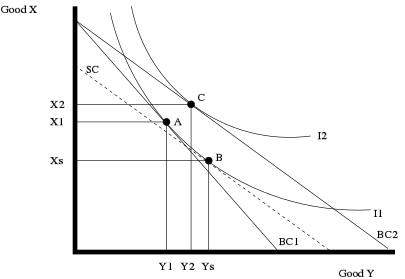
The substitution effect, , is the change in the amount demanded for when the price of good falls from to (represented by the budget constraint shifting from BC1 to BC2 and thus increasing purchasing power) and, at the same time, the money income falls from to to keep the consumer at the same level of utility on :
The substitution effect increases the amount demanded of good from to in the diagram. In the example shown, the income effect of the fall in partly offsets the substitution effect as the amount demanded of in the absence of an offsetting income change ends up at thus the income effect from the rise in purchasing power due to the price drop is that the quantity demanded of goes from to . The total effect of the price drop on quantity demanded is the sum of the substitution effect and the income effect.
Assumptions
The behavioral assumption of the consumer theory proposed herein is that all consumers seek to maximize utility. In the mainstream economics tradition, this activity of maximizing utility has been deemed as the "rational" behavior of decision makers. More specifically, in the eyes of economists, all consumers seek to maximize a utility function subject to a budgetary constraint.[4] In other words, economists assume that consumers will always choose the "best" bundle of goods they can afford.[5] Consumer theory is therefore based on generating refutable hypotheses about the nature of consumer demand from this behavioral postulate.[4]
In order to reason from the central postulate towards a useful model of consumer choice, it is necessary to make additional assumptions about the certain preferences that consumers employ when selecting their preferred "bundle" of goods. These are relatively strict, allowing for the model to generate more useful hypotheses with regard to consumer behaviour than weaker assumptions, which would allow any empirical data to be explained in terms of stupidity, ignorance, or some other factor, and hence would not be able to generate any predictions about future demand at all.[4] For the most part, however, they represent statements which would only be contradicted if a consumer was acting in (what was widely regarded as) a strange manner.[6] In this vein, the modern form of consumer choice theory assumes:
- Preferences are complete
- Consumer choice theory is based on the assumption that the consumer fully understands his or her own preferences, allowing for a simple but accurate comparison between any two bundles of good presented.[5] That is to say, it is assumed that if a consumer is presented with two consumption bundles A and B each containing different combinations of n goods, the consumer can unambiguously decide if (s)he prefers A to B, B to A, or is indifferent to both.[4][5] The few scenarios where it is possible to imagine that decision-making would be very difficult are thus placed "outside the domain of economic analysis".[5] However, discoveries in behavioral economics has found that actual decision making is affected by various factors, such as whether choices are presented together or separately through the distinction bias.
- Preferences are reflexive
- Means that if A and B are in all respect identical the consumer will consider A to be at least as good as (i.e. weakly preferred to) B.[5] Alternatively, the axiom can be modified to read that the consumer is indifferent with regard to A and B.[7]
- Preference are transitive
- If A is preferred to B and B is preferred to C then A must be preferred to C.
- This also means that if the consumer is indifferent between A and B and is indifferent between B and C she will be indifferent between A and C.
- This is the consistency assumption. This assumption eliminates the possibility of intersecting indifference curves.
- Preferences exhibit non-satiation
- This is the "more is always better" assumption; that in general if a consumer is offered two almost identical bundles A and B, but where B includes more of one particular good, the consumer will choose B.[8]
- Among other things this assumption precludes circular indifference curves. Non-satiation in this sense is not a necessary but a convenient assumption. It avoids unnecessary complications in the mathematical models.
- Indifference curves exhibit diminishing marginal rates of substitution
- This assumption assures that indifference curves are smooth and convex to the origin.
- This assumption is implicit in the last assumption.
- This assumption also set the stage for using techniques of constrained optimization. Because the shape of the curve assures that the first derivative is negative and the second is positive.
- The MRS tells how much y a person is willing to sacrifice to get one more unit of x.
- This assumption incorporates the theory of diminishing marginal utility.
- Goods are available in all quantities
- It is assumed that a consumer may choose to purchase any quantity of a good (s)he desires, for example, 2.6 eggs and 4.23 loaves of bread. Whilst this makes the model less precise, it is generally acknowledged to provide a useful simplification to the calculations involved in consumer choice theory, especially since consumer demand is often examined over a considerable period of time. The more spending rounds are offered, the better approximation the continuous, differentiable function is for its discrete counterpart. (Whilst the purchase of 2.6 eggs sounds impossible, an average consumption of 2.6 eggs per day over a month does not.)[8]
Note the assumptions do not guarantee that the demand curve will be negatively sloped. A positively sloped curve is not inconsistent with the assumptions.[9]
Use value
In Marx's critique of political economy, any labor-product has a value and a use value, and if it is traded as a commodity in markets, it additionally has an exchange value, most often expressed as a money-price.[10] Marx acknowledges that commodities being traded also have a general utility, implied by the fact that people want them, but he argues that this by itself tells us nothing about the specific character of the economy in which they are produced and sold.
Labor-leisure tradeoff
One can also use consumer theory to analyze a consumer's choice between leisure and labor. Leisure is considered one good (often put on the horizontal axis) and consumption is considered the other good. Since a consumer has a finite amount of time, he must make a choice between leisure (which earns no income for consumption) and labor (which does earn income for consumption).
The previous model of consumer choice theory is applicable with only slight modifications. First, the total amount of time that an individual has to allocate is known as his "time endowment", and is often denoted as T. The amount an individual allocates to labor (denoted L) and leisure (ℓ) is constrained by T such that
A person's consumption is the amount of labor they choose multiplied by the amount they are paid per hour of labor (their wage, often denoted w). Thus, the amount that a person consumes is:
When a consumer chooses no leisure then and .
From this labor-leisure tradeoff model, the substitution effect and income effect from various changes caused by welfare benefits, labor taxation, or tax credits can be analyzed.
See also
- Convex preferences
- Consumer sovereignty
- Consumerism
- Important publications in consumer theory
- Indifference curves
- Microeconomics
- Opportunity cost
- Producer theory – the dual of consumer theory
- Supply and demand
- Utility maximization problem
References
- "What is 'consumer choice theory'? — Economy". Economy. Retrieved 2017-05-31.
- Silberberg & Suen 2001, p. 255
- Berliant, M.; Raa, T. T. (1988). "A foundation of location theory: Consumer preferences and demand". Journal of Economic Theory. 44 (2): 336. doi:10.1016/0022-0531(88)90008-7.
- Silberberg & Suen 2001, pp. 252–254
- Varian 2006, p. 20
- Silberberg & Suen 2001, p. 260
- Binger & Hoffman 1998, pp. 109–17
- Silberberg & Suen 2001, pp. 256–257
- Binger & Hoffman 1998, pp. 141–143
- "Glossary of Terms: Us". Marxists.org. Retrieved 2013-11-07.
- Silberberg; Suen (2001). The Structure of Economics, A Mathematical Analysis. McGraw-Hill.CS1 maint: ref=harv (link)
- Böhm, Volker; Haller, Hans (1987). "Demand theory". The New Palgrave: A Dictionary of Economics. 1. pp. 785–92.CS1 maint: ref=harv (link)
- Hicks, John R. (1946) [1939]. Value and Capital (2nd ed.).CS1 maint: ref=harv (link)
- Binger; Hoffman (1998). Microeconomics with Calculus (2nd ed.). Addison Wesley. pp. 141–43.CS1 maint: ref=harv (link)
External links
