Real business-cycle theory
Real business-cycle theory (RBC theory) is a class of new classical macroeconomics models in which business-cycle fluctuations to a large extent can be accounted for by real (in contrast to nominal) shocks. Unlike other leading theories of the business cycle, RBC theory sees business cycle fluctuations as the efficient response to exogenous changes in the real economic environment. That is, the level of national output necessarily maximizes expected utility, and governments should therefore concentrate on long-run structural policy changes and not intervene through discretionary fiscal or monetary policy designed to actively smooth out economic short-term fluctuations.
According to RBC theory, business cycles are therefore "real" in that they do not represent a failure of markets to clear but rather reflect the most efficient possible operation of the economy, given the structure of the economy.
RBC theory is associated with freshwater economics (the Chicago School of Economics in the neoclassical tradition).
Business cycles
If we were to take snapshots of an economy at different points in time, no two photos would look alike. This occurs for two reasons:
- Many advanced economies exhibit sustained growth over time. That is, snapshots taken many years apart will most likely depict higher levels of economic activity in the later period.
- There exist seemingly random fluctuations around this growth trend. Thus given two snapshots in time, predicting the latter with the earlier is nearly impossible.
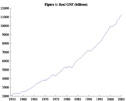
A common way to observe such behavior is by looking at a time series of an economy's output, more specifically gross national product (GNP). This is just the value of the goods and services produced by a country's businesses and workers.
Figure 1 shows the time series of real GNP for the United States from 1954–2005. While we see continuous growth of output, it is not a steady increase. There are times of faster growth and times of slower growth. Figure 2 transforms these levels into growth rates of real GNP and extracts a smoother growth trend. A common method to obtain this trend is the Hodrick–Prescott filter. The basic idea is to find a balance between the extent to which general growth trend follows the cyclical movement (since long term growth rate is not likely to be perfectly constant) and how smooth it is. The HP filter identifies the longer term fluctuations as part of the growth trend while classifying the more jumpy fluctuations as part of the cyclical component.
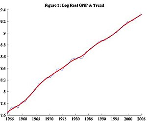
Observe the difference between this growth component and the jerkier data. Economists refer to these cyclical movements about the trend as business cycles. Figure 3 explicitly captures such deviations. Note the horizontal axis at 0. A point on this line indicates at that year, there is no deviation from the trend. All other points above and below the line imply deviations. By using log real GNP the distance between any point and the 0 line roughly equals the percentage deviation from the long run growth trend. Also note that the Y-axis uses very small values. This indicates that the deviations in real GNP are very small comparatively, and might be attributable to measurement errors rather than real deviations.
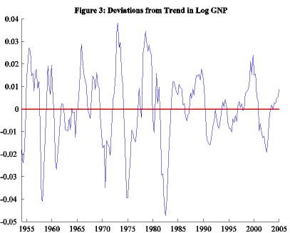
We call large positive deviations (those above the 0 axis) peaks. We call relatively large negative deviations (those below the 0 axis) troughs. A series of positive deviations leading to peaks are booms and a series of negative deviations leading to troughs are recessions.
At a glance, the deviations just look like a string of waves bunched together—nothing about it appears consistent. To explain causes of such fluctuations may appear rather difficult given these irregularities. However, if we consider other macroeconomic variables, we will observe patterns in these irregularities. For example, consider Figure 4 which depicts fluctuations in output and consumption spending, i.e. what people buy and use at any given period. Observe how the peaks and troughs align at almost the same places and how the upturns and downturns coincide.
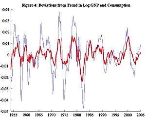
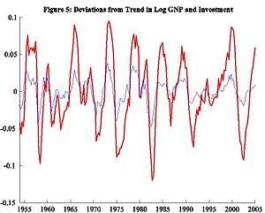
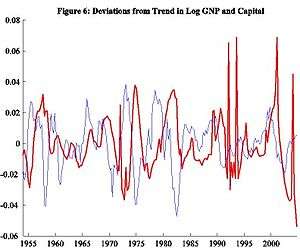
We might predict that other similar data may exhibit similar qualities. For example, (a) labor, hours worked (b) productivity, how effective firms use such capital or labor, (c) investment, amount of capital saved to help future endeavors, and (d) capital stock, value of machines, buildings and other equipment that help firms produce their goods. While Figure 5 shows a similar story for investment, the relationship with capital in Figure 6 departs from the story. We need a way to pin down a better story; one way is to look at some statistics.
Stylized facts
By eyeballing the data, we can infer several regularities, sometimes called stylized facts. One is persistence. For example, if we take any point in the series above the trend (the x-axis in figure 3), the probability the next period is still above the trend is very high. However, this persistence wears out over time. That is, economic activity in the short run is quite predictable but due to the irregular long-term nature of fluctuations, forecasting in the long run is much more difficult if not impossible.
Another regularity is cyclical variability. Column A of Table 1 lists a measure of this with standard deviations. The magnitude of fluctuations in output and hours worked are nearly equal. Consumption and productivity are similarly much smoother than output while investment fluctuates much more than output. The capital stock is the least volatile of the indicators.
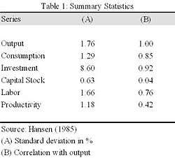
Yet another regularity is the co-movement between output and the other macroeconomic variables. Figures 4 – 6 illustrated such relationship. We can measure this in more detail using correlations as listed in column B of Table 1. Procyclical variables have positive correlations since it usually increases during booms and decreases during recessions. Vice versa, a countercyclical variable associates with negative correlations. Acyclical, correlations close to zero, implies no systematic relationship to the business cycle. We find that productivity is slightly procyclical. This implies workers and capital are more productive when the economy is experiencing a boom. They are not quite as productive when the economy is experiencing a slowdown. Similar explanations follow for consumption and investment, which are strongly procyclical. Labor is also procyclical while capital stock appears acyclical.
Observing these similarities yet seemingly non-deterministic fluctuations about trend, the question arises as to why any of this occurs. Since people prefer economic booms over recessions, it follows that if all people in the economy make optimal decisions, these fluctuations are caused by something outside the decision-making process. So the key question really is: what main factor influences and subsequently changes the decisions of all factors in an economy?
Economists have come up with many ideas to answer the above question. The one which currently dominates the academic literature on real business cycle theory was introduced by Finn E. Kydland and Edward C. Prescott in their 1982 work Time to Build And Aggregate Fluctuations. They envisioned this factor to be technological shocks—i.e., random fluctuations in the productivity level that shifted the constant growth trend up or down. Examples of such shocks include innovations, bad weather, imported oil price increase, stricter environmental and safety regulations, etc. The general gist is that something occurs that directly changes the effectiveness of capital and/or labour. This in turn affects the decisions of workers and firms, who in turn change what they buy and produce and thus eventually affect output. RBC models predict time sequences of allocation for consumption, investment, etc. given these shocks.
But exactly how do these productivity shocks cause ups and downs in economic activity? Consider a positive but temporary shock to productivity. This momentarily increases the effectiveness of workers and capital, allowing a given level of capital and labor to produce more output.
Individuals face two types of tradeoffs. One is the consumption-investment decision. Since productivity is higher, people have more output to consume. An individual might choose to consume all of it today. But if he values future consumption, all that extra output might not be worth consuming in its entirety today. Instead, he may consume some but invest the rest in capital to enhance production in subsequent periods and thus increase future consumption. This explains why investment spending is more volatile than consumption. The life-cycle hypothesis argues that households base their consumption decisions on expected lifetime income and so they prefer to "smooth" consumption over time. They will thus save (and invest) in periods of high income and defer consumption of this to periods of low income.
The other decision is the labor-leisure tradeoff. Higher productivity encourages substitution of current work for future work since workers will earn more per hour today compared to tomorrow. More labor and less leisure results in higher output today. greater consumption and investment today. On the other hand, there is an opposing effect: since workers are earning more, they may not want to work as much today and in future periods. However, given the pro-cyclical nature of labor, it seems that the above substitution effect dominates this income effect.
Overall, the basic RBC model predicts that given a temporary shock, output, consumption, investment and labor all rise above their long-term trends and hence formulate into a positive deviation. Furthermore, since more investment means more capital is available for the future, a short-lived shock may have an impact in the future. That is, above-trend behavior may persist for some time even after the shock disappears. This capital accumulation is often referred to as an internal "propagation mechanism", since it may increase the persistence of shocks to output.
A string of such productivity shocks will likely result in a boom. Similarly, recessions follow a string of bad shocks to the economy. If there were no shocks, the economy would just continue following the growth trend with no business cycles.
To quantitatively match the stylized facts in Table 1, Kydland and Prescott introduced calibration techniques. Using this methodology, the model closely mimics many business cycle properties. Yet current RBC models have not fully explained all behavior and neoclassical economists are still searching for better variations.
The main assumption in RBC theory is that individuals and firms respond optimally all the time. It follows that business cycles exhibited in an economy are chosen in preference to no business cycles at all. This is not to say that people like to be in a recession. Slumps are preceded by an undesirable productivity shock which constrains the situation. But given these new constraints, people will still achieve the best outcomes possible and markets will react efficiently. So when there is a slump, people are choosing to be in that slump because given the situation, it is the best solution. This suggests laissez-faire (non-intervention) is the best policy of government towards the economy but given the abstract nature of the model, this has been debated.
A precursor to RBC theory was developed by monetary economists Milton Friedman and Robert Lucas in the early 1970s. They envisioned the factor that influenced people's decisions to be misperception of wages —that booms and recessions occurred when workers perceived wages higher or lower than they really were. This meant they worked and consumed more or less than otherwise. In a world of perfect information, there would be no booms or recessions.
Calibration
Unlike estimation, which is usually used for the construction of economic models, calibration only returns to the drawing board to change the model in the face of overwhelming evidence against the model being correct; this inverts the burden of proof away from the builder of the model. In fact, simply stated, it is the process of changing the model to fit the data. Since RBC models explain data ex post, it is very difficult to falsify any one model that could be hypothesised to explain the data. RBC models are highly sample specific, leading some to believe that they have little or no predictive power.
Structural variables
Crucial to RBC models, "plausible values" for structural variables such as the discount rate, and the rate of capital depreciation are used in the creation of simulated variable paths. These tend to be estimated from econometric studies, with 95% confidence intervals. If the full range of possible values for these variables is used, correlation coefficients between actual and simulated paths of economic variables can shift wildly, leading some to question how successful a model which only achieves a coefficient of 80% really is.
Criticisms
The real business cycle theory relies on three assumptions which according to economists such as Greg Mankiw and Larry Summers are unrealistic:[1]
1. The model is driven by large and sudden changes in available production technology.
- Summers noted that Prescott is unable to suggest any specific technological shock for an actual downturn apart from the oil price shock in the 1970s.[2] Furthermore there is no microeconomic evidence for the large real shocks that need to drive these models. Real business cycle models as a rule are not subjected to tests against competing alternatives[3] which are easy to support.(Summers 1986)
2. Unemployment reflects changes in the amount people want to work.
- Paul Krugman argued that this assumption would mean that 25% unemployment at the height of the Great Depression (1933) would be the result of a mass decision to take a long vacation.[4]
3. Monetary policy is irrelevant for economic fluctuations.
- Nowadays it is widely agreed that wages and prices do not adjust as quickly as needed to restore equilibrium. Therefore most economists, even among the new classicists, do not accept the policy-ineffectiveness proposition.[4]
Another major criticism is that real business cycle models can not account for the dynamics displayed by U.S. gross national product.[5] As Larry Summers said: "(My view is that) real business cycle models of the type urged on us by [Ed] Prescott have nothing to do with the business cycle phenomena observed in the United States or other capitalist economies." —(Summers 1986)
See also
References
- Cencini, Alvaro (2005). Macroeconomic Foundations of Macroeconomics. Routledge. p. 40. ISBN 978-0-415-31265-3.
- Summers, Lawrence H. (Fall 1986). "Some Skeptical Observations on Real Business Cycle Theory" (PDF). Federal Reserve Bank of Minneapolis Quarterly Review. 10 (4): 23–27.
- George W. Stadler, Real Business Cycles, Journal of Economics Literatute, Vol. XXXII, December 1994, pp. 1750–1783, see p. 1772
- Kevin Hoover (2008). "New Classical Macroeconomics", econlib.org
- George W. Stadler, Real Business Cycles, Journal of Economics Literatute, Vol. XXXII, December 1994, pp. 1750–1783, see p. 1769
Further reading
- Cooley, Thomas F. (1995). Frontiers of Business Cycle Research. Princeton: Princeton University Press. ISBN 978-0-691-04323-4.
- Gomes, Joao; Greenwood, Jeremy; Rebelo, Sergio (2001). "Equilibrium Unemployment". Journal of Monetary Economics. 48 (1): 109–152. doi:10.1016/S0304-3932(01)00071-X.
- Hansen, Gary D. (1985). "Indivisible labor and the business cycle". Journal of Monetary Economics. 16 (3): 309–327. CiteSeerX 10.1.1.335.3000. doi:10.1016/0304-3932(85)90039-X.
- Heijdra, Ben J. (2009). "Real Business Cycles". Foundations of Modern Macroeconomics (2nd ed.). Oxford: Oxford University Press. pp. 495–552. ISBN 978-0-19-921069-5.
- Kydland, Finn E.; Prescott, Edward C. (1982). "Time to Build and Aggregate Fluctuations". Econometrica. 50 (6): 1345–1370. doi:10.2307/1913386. JSTOR 1913386.
- Long, John B., Jr.; Plosser, Charles (1983). "Real Business Cycles". Journal of Political Economy. 91 (1): 39–69. doi:10.1086/261128.
- Lucas, Robert E., Jr. (1977). "Understanding Business Cycles". Carnegie-Rochester Conference Series on Public Policy. 5: 7–29. doi:10.1016/0167-2231(77)90002-1.
- Plosser, Charles I. (1989). "Understanding real business cycles". Journal of Economic Perspectives. 3 (3): 51–77. doi:10.1257/jep.3.3.51. JSTOR 1942760.
- Romer, David (2011). "Real-Business-Cycle Theory". Advanced Macroeconomics (Fourth ed.). New York: McGraw-Hill. pp. 189–237. ISBN 978-0-07-351137-5.
