Fisher transformation

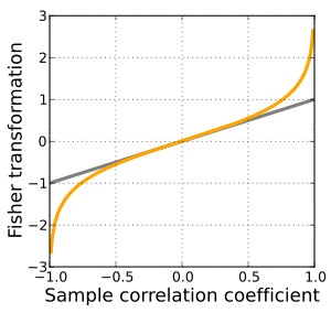
In statistics, the Fisher transformation (aka Fisher z-transformation) can be used to test hypotheses about the value of the population correlation coefficient ρ between variables X and Y.[1][2] This is because, when the transformation is applied to the sample correlation coefficient, the sampling distribution of the resulting variable is approximately normal, with a variance that is stable over different values of the underlying true correlation.

"Fisher z-transformation" redirects here. It is not to be confused with Fisher's z-distribution.

For standard z-score in statistics, see Standard score. For z-transformation to complex number domain, see Z-transform.

A graph of the transformation (in orange). The untransformed sample correlation coefficient is plotted on the horizontal axis, and the transformed coefficient is plotted on the vertical axis. The identity function (gray) is also shown for comparison.

Definition

Given a set of N bivariate sample pairs (X_i, Y_i), i = 1, ..., N, the sample correlation coefficient r is given by

${\displaystyle r={\frac {\operatorname {cov} (X,Y)}{\sigma _{X}\sigma _{Y}}}={\frac {\sum _{i=1}^{N}(X_{i}-{\bar {X}})(Y_{i}-{\bar {Y}})}{{\sqrt {\sum _{i=1}^{N}(X_{i}-{\bar {X}})^{2}}}{\sqrt {\sum _{i=1}^{N}(Y_{i}-{\bar {Y}})^{2}}}}}.}$

Here ${\displaystyle \operatorname {cov} (X,Y)}$ stands for the covariance between the variables ${\displaystyle X}$ and ${\displaystyle Y}$ and ${\displaystyle \sigma }$ stands for the standard deviation of the respective variable. Fisher's z-transformation of r is defined as

${\displaystyle z={1 \over 2}\ln \left({1+r \over 1-r}\right)=\operatorname {arctanh} (r),}$

where "ln" is the natural logarithm function and "arctanh" is the inverse hyperbolic tangent function.

If (X, Y) has a bivariate normal distribution with correlation ρ and the pairs (X_i, Y_i) are independent and identically distributed, then z is approximately normally distributed with mean

${\displaystyle {1 \over 2}\ln \left({{1+\rho } \over {1-\rho }}\right),}$

and standard error

${\displaystyle {1 \over {\sqrt {N-3}}},}$

where N is the sample size, and ρ is the true correlation coefficient.

This transformation, and its inverse

${\displaystyle r={\frac {\exp(2z)-1}{\exp(2z)+1}}=\operatorname {tanh} (z),}$

can be used to construct a large-sample confidence interval for r using standard normal theory and derivations. See also application to partial correlation.

Derivation

Fisher Transformation with ${\displaystyle \rho =0.9}$ and ${\displaystyle N=30}$. Illustrated is the exact probability density function of ${\displaystyle r}$ (in black), together with the probability density functions of the usual Fisher transformation (blue) and that obtained by including extra terms that depend on ${\displaystyle N}$ (red). The latter approximation is visually indistinguishable from the exact answer (its maximum error is 0.3%, compared to 3.4% of basic Fisher).

To derive the Fisher transformation, one starts by considering an arbitrary increasing function of ${\displaystyle r}$, say ${\displaystyle G(r)}$. Finding the first term in the large-${\displaystyle N}$ expansion of the corresponding skewness results in

${\displaystyle {\frac {6\rho -3(1-\rho ^{2})G^{\prime \prime }(\rho )/G^{\prime }(\rho )}{\sqrt {N}}}+O(N^{-3/2}).}$

Making it equal to zero and solving the corresponding differential equation for ${\displaystyle G}$ yields the ${\displaystyle \operatorname {artanh} }$ function. Similarly expanding the mean and variance of ${\displaystyle \operatorname {artanh} (r)}$, one gets

${\displaystyle \operatorname {artanh} (\rho )+{\frac {\rho }{2N}}+O(N^{-2})}$

and

${\displaystyle {\frac {1}{N}}+{\frac {6-\rho ^{2}}{2N^{2}}}+O(N^{-3})}$

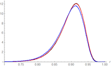
respectively. The extra terms are not part of the usual Fisher transformation. For large values of ${\displaystyle \rho }$ and small values of ${\displaystyle N}$ they represent a large improvement of accuracy at minimal cost, although they greatly complicate the computation of the inverse as a closed-form expression is not available. The near-constant variance of the transformation is the result of removing its skewness – the actual improvement is achieved by the latter, not by the extra terms. Including the extra terms yields:

${\displaystyle {\frac {z-\operatorname {artanh} (\rho )-{\frac {\rho }{2N}}}{\sqrt {{\frac {1}{N}}+{\frac {6-\rho ^{2}}{2N^{2}}}}}}}$

which has, to an excellent approximation, a standard normal distribution.[3]

Discussion

The Fisher transformation is an approximate variance-stabilizing transformation for r when X and Y follow a bivariate normal distribution. This means that the variance of z is approximately constant for all values of the population correlation coefficient ρ. Without the Fisher transformation, the variance of r grows smaller as |ρ| gets closer to 1. Since the Fisher transformation is approximately the identity function when |r| < 1/2, it is sometimes useful to remember that the variance of r is well approximated by 1/N as long as |ρ| is not too large and N is not too small. This is related to the fact that the asymptotic variance of r is 1 for bivariate normal data.

The behavior of this transform has been extensively studied since Fisher introduced it in 1915. Fisher himself found the exact distribution of z for data from a bivariate normal distribution in 1921; Gayen in 1951[4] determined the exact distribution of z for data from a bivariate Type A Edgeworth distribution. Hotelling in 1953 calculated the Taylor series expressions for the moments of z and several related statistics[5] and Hawkins in 1989 discovered the asymptotic distribution of z for data from a distribution with bounded fourth moments.[6]

Other uses

While the Fisher transformation is mainly associated with the Pearson product-moment correlation coefficient for bivariate normal observations, it can also be applied to Spearman's rank correlation coefficient in more general cases.[7] A similar result for the asymptotic distribution applies, but with a minor adjustment factor: see the latter article for details.

See also

• Data transformation (statistics)
• Meta-analysis (this transformation is used in meta analysis for stabilizing the variance)
• Partial correlation
• R implementation

References

1. Fisher, R. A. (1915). "Frequency distribution of the values of the correlation coefficient in samples of an indefinitely large population". Biometrika. 10 (4): 507–521. doi:10.2307/2331838. hdl:2440/15166. JSTOR 2331838.
2. Fisher, R. A. (1921). "On the 'probable error' of a coefficient of correlation deduced from a small sample" (PDF). Metron. 1: 3–32.
3. Vrbik, Jan (December 2005). "Population moments of sampling distributions". Computational Statistics. 20 (4): 611–621. doi:10.1007/BF02741318.
4. Gayen, A. K. (1951). "The Frequency Distribution of the Product-Moment Correlation Coefficient in Random Samples of Any Size Drawn from Non-Normal Universes". Biometrika. 38 (1/2): 219–247. doi:10.1093/biomet/38.1-2.219. JSTOR 2332329.
5. Hotelling, H (1953). "New light on the correlation coefficient and its transforms". Journal of the Royal Statistical Society, Series B. 15 (2): 193–225. JSTOR 2983768.
6. Hawkins, D. L. (1989). "Using U statistics to derive the asymptotic distribution of Fisher's Z statistic". The American Statistician. 43 (4): 235–237. doi:10.2307/2685369. JSTOR 2685369.
7. Zar, Jerrold H. (2005). Spearman Rank Correlation: Overview. Encyclopedia of Biostatistics. doi:10.1002/9781118445112.stat05964. ISBN 9781118445112.