Linear form

In linear algebra, a linear form (also known as a linear functional, a one-form, or a covector) is a linear map from a vector space to its field of scalars. In ℝⁿ, if vectors are represented as column vectors, then linear functionals are represented as row vectors, and their action on vectors is given by the matrix product with the row vector on the left and the column vector on the right. In general, if V is a vector space over a field k, then a linear functional f is a function from V to k that is linear:

f({\vec {v}}+{\vec {w}})=f({\vec {v}})+f({\vec {w}})

for all

{\vec {v}},{\vec {w}}\in V

f(a{\vec {v}})=af({\vec {v}})

for all

{\vec {v}}\in V,a\in k.

The set of all linear functionals from V to k, denoted by Hom_k(V,k), forms a vector space over k with the operations of addition and scalar multiplication defined pointwise. This space is called the dual space of V, or sometimes the algebraic dual space, to distinguish it from the continuous dual space. It is often written V^∗, V′, or V^ᐯ when the field k is understood.

Linear functionals on real or complex vector spaces

We assume throughout that all vector spaces that we consider are either vector spaces over the set of real numbers $ℝ$ or vector spaces over the set of complex numbers $ℂ$ .

We assume that $X$ is a vector space over $𝕂$ where $𝕂$ is either $ℝ$ or $ℂ$ .

Basic definitions

Definition: If

X

is a vector space over a field

𝕂

then

𝕂

is called

X

's underlying (scalar) field and any element of

𝕂

is called a scalar.

Definition: A linear map is a map

F : X \to Y

between two vector spaces

X

and

Y

that have the same underlying scalar field, such that

F (x + sy) = F (x) + sF (y)

for all

x, y \in X

and all scalars

s

. If

X

and

Y

do not necessarily have the same underlying scalar field then we say that

F

is $ℝ$ -linear and is a linear map over $ℝ$ if it is a linear map when

X

and

Y

are both considered as vector spaces over

ℝ

(i.e. if

F (x + ry) = F (x) + rF (y)

for all

x, y \in X

and all real

r

).

Definition: The kernel of a map

F

on

X

is the set

Ker F := {x \in X : F (x) = 0

}. We say that a map is trivial if it is identically equal to 0.

Definition: A functional on a vector space

X

is a map from

X

into

X

's underlying field. A linear functional on

X

is a functional that is also a linear map.

Observe that if $X$ is a vector space over $ℝ$ then a "linear functional on $X$ " is a linear map of the form $f : X \to ℝ$ (valued in $ℝ$ ), while if $X$ is a vector space over $ℂ$ then a "linear functional on $X$ " is a linear map of the form $f : X \to ℂ$ (valued in $ℂ$ ).

Recall that $ℝ$ (resp. $ℂ$ ) is a vector space over $ℝ$ (resp. $ℂ$ ) so we can ask what are the linear functionals on $ℝ$ ? A function $f : ℝ \to ℝ$ is a linear functional on $X = ℝ$ if and only if it is of the form $f (x) = rx$ for some real number $r \in ℝ$ . Note in particular that a function $f$ having the equation of a line $f (x) = a + rx$ with $a \neq 0$ (e.g. $f (x) = 1 + 2 x$ ) is not a linear functional on $ℝ$ (since for instance, $f (1 + 1) = a + 2 r \neq 2 a + 2 r = f (1) + f (1)$ ). It is however, a type of function known as an affine linear functional.

A linear functional $f$ is non-trivial if and only if it is surjective (i.e. its range is all of $𝕂$ ).[1]

Definition: The algebraic dual space, or simply the dual space, is the vector space over

𝕂

consisting of all linear functionals on

X

. It will be denoted by

X #

.

Definition: If

f

and

g

are two real-valued functions and if

S

is a set that belongs to both of their domains, then we say that

g

dominates

f

on

S

and write $f \leq g$ on $S$ if

f (s) \leq g (s)

for all

s \in S

. We say that

g

extends

f

if every

x

in the domain of

f

belongs to the domain of

g

and

f (x) = g (x)

. If

g

extends

f

then we call

g

a linear extension of

f

if

g

is a linear map.

Relationships with other maps

Relationship between real and complex linear functionals

Suppose that $X$ is a vector space over $ℂ$ . Let $X ℝ$ denote $X$ when it is considered as a vector space over $ℝ$ . Note that every linear functional on $X$ is, by definition, complex-valued while every linear functional on $X ℝ$ is real-valued.

Definition: By a real linear functional on

X

, we mean a linear functional on

X ℝ

(i.e. a linear map of the form

f : X ℝ \to ℝ

, or more explicitly, a map

f : X \to ℝ

such that

f (x + y) = f (x) + f (y)

and

f (rx) = r f (x)

for all

x, y \in X

and all real

r \in ℝ

).

If $g$ is a real linear functional on $X$ then $g$ is a linear functional on $X$ if and only if $g$ is trivial (i.e. if $g \in X ℝ #$ then $g \in X #$ if and only if $g = 0$ ) (see footnote for an explanation).[2] Thus, we note the following important technicality:

WARNING: Any non-trivial linear functional on a complex vector space

X

is not a real linear functional on

X

. And conversely, any non-trivial real linear functional on a complex vector space

X

is not a linear functional on

X

. However, on a real vector space, linear functionals and real linear functionals are one and the same.

However, a real linear functional $g$ on $X$ does induce a canonical linear functional $L g \in X #$ defined by $L g (x) := g (x) - i g (ix)$ for all $x \in X$ , where $i := \sqrt -1$ .

Now suppose that $f \in X #$ and let $R := Re f$ (resp. $I := Im f$ ) denote the real (resp. imaginary) part of $f$ so that $f (x) = R (x) + i I (x)$ . Then for all $x \in X$ , $I (x) = - R (ix)$ and $R (x) = I (ix)$ so that

f (x) = R (x) - i R (ix) = I (ix) + i I (x)

.

This shows that $f$ , $R$ , and $I$ each completely determine one another[3] and it follows that $R$ and $I$ are real linear functionals on $X$ and the canonical linear functional on $X$ induced by $R$ is $f$ (i.e. $L R = f$ ). Furthermore, for all $x \in X$ ,

| f (x) | 2 = | R (ix) | 2 + | R (x) | 2 = | I (ix) | 2 + | I (x) | 2

= | R (ix) | 2 + | I (ix) | 2 = | R (x) | 2 + | I (x) | 2

.

Thus the map $g \mapsto L g$ , denoted by $L •$ , defines a one-to-one correspondence from $X ℝ #$ onto $X #$ whose inverse is the map $f \mapsto Re f$ . Furthermore, $L •$ is linear as a map over $ℝ$ (i.e. $L g + h = L g + L h$ and $L rg = r L g$ for all $r \in ℝ$ and $g, h \in X ℝ #$ ). Similarly, the inverse of the surjective map $X # \to X ℝ #$ defined by $f \mapsto Im f$ is the map $X ℝ # \to X #$ that sends $I \in X ℝ #$ to the linear functional $x \mapsto I (ix) + i I (x)$ .

This relationship was discovered by Henry Löwig in 1934 (although it is usually credited to F. Murray).[4]

If $f$ is a linear functional on a real or complex vector space $X$ and if $p$ is a seminorm on $X$ , then $| f | \leq p$ on $X$ if and only if $Re f \leq p$ on $X$ (see footnote for proof).[5][6]

Topological consequences

If $X$ is a complex topological vector space (TVS), then either all three of $f$ , $Re f$ , and $Im f$ are continuous (resp. bounded), or else all three are discontinuous (resp. unbounded). Moreover, if $X$ is a complex normed space then $| | f | | = | | Re f | |$ [7] (where in particular, one side is infinite if and only if the other side is infinite).

Relationships with seminorms and sublinear functions

A sublinear function on a vector space $X$ is a function $p : X \to ℝ$ that satisfies the following two properties:

Subadditivity: $p (x + y) \leq p (x) + p (y)$ for all $x, y \in X$ ;
Positive homogeneity: $p (rx) = r p (x)$ for any positive real $r > 0$ and any $x \in X$ .

A seminorm on $X$ is a sublinear function $p : X \to ℝ$ that satisfies the following additional property:

Absolute homogeneity: $p (sx) = | s | p (x)$ for all $x \in X$ and all scalars $s$ ;

Note that every linear functional on a real vector space is a sublinear function, although there are sublinear functions that are not linear functionals. Unlike linear functionals, a seminorm $p$ is valued in the non-negative real numbers (i.e. $p (x)$ is a real number and $p (x) \geq 0$ ), so the only linear function that is also a seminorm is the trivial (identically) 0 map. However, if $f$ is a linear functional on a vector space $X$ , then its absolute value is a seminorm on $X$ (i.e. the map on $X$ defined by $p f (x) := | f(x) |$ for all $x \in X$ is a seminorm on $X$ )

If $f$ is a linear functional on a real vector space $X$ and $p$ is a seminorm on $X$ , then $f \leq p$ if and only if $| f | \leq p$ .[8]

Hahn-Banach theorem

The Hahn-Banach theorem is considered one of the most important results of the subfield of mathematics called functional analysis (as the name suggests, linear functionals play an important role in functional analysis). Due to its importance, the Hahn-Banach theorem has been generalized many times and today "Hahn-Banach theorem" refers to any one of a collection of theorems. The general idea behind a Hahn-Banach theorem is that it gives conditions under which a linear functional on a vector subspace $M$ of $X$ (satisfying a certain condition) can be extended to a linear functional on the whole of $X$ (that continues to satisfy that condition). The following is one of many results known collectively as "Hahn-Banach theorems."

Hahn–Banach dominated extension theorem[3](Rudin 1991, Th. 3.2) — If $p : X \to ℝ$ is a sublinear function, and $f : M \to ℝ$ is a linear functional on a linear subspace $M \subseteq X$ which is dominated by $p$ on $M$ , then there exists a linear extension $F : X \to ℝ$ of $f$ to the whole space $X$ that is dominated by $p$ , i.e., there exists a linear functional $F$ such that

F (m) = f (m)

for all

m \in M

,

| F (x) | \leq p (x)

for all

x \in X

.

Relationships between multiple linear functionals

Any two linear functionals with the same kernel are proportional (i.e. scalar multiples of each other). This fact can be generalized to the following theorem.

Theorem[9][10] — If $f, g 1, ..., g n$ are linear functionals on $X$ , then the following are equivalent:

$f$ can be written as a linear combination of $g 1, ..., g n$ (i.e. there exist scalars $s 1, ..., s n$ such that $f = s 1 g 1 + \cdot\cdot\cdot + s n g n$ );
$\cap n i =1 Ker g i \subseteq Ker f$ ;
there exists a real number $r$ such that $| f (x) | \leq r | g i (x) |$ for all $x \in X$ and all $i$ .

If $f$ is a non-trivial linear functional on $X$ with kernel $N$ , $x \in X$ satisfies $f (x) = 1$ , and $U$ is a balanced subset of $X$ , then $N \cap (x + U) = \emptyset$ if and only if $| f (u)| < 1$ for all $u \in U$ .[7]

Hyperplanes and maximal subspaces

Definition:[4] A vector subspace

M

of a vector space

X

is called proper if

M \neq X

and it is called maximal in

X

if it is proper and the only vector subspace of

X

that contains

M

is

X

itself.

Definition:[4] A hyperplane in

X

is a translate of a maximal vector subspace (i.e. it is a set of the form

x + M := {x + m : m \in M

} where

M

is a maximal vector subspace of

X

and

x

is any element of

X

.

A vector subspace $M$ of $X$ is maximal in $X$ if and only if it is the kernel of some non-trivial linear functional on $X$ (i.e. $M = ker f$ for some non-trivial linear functional $f$ on $X$ ).[4]

A vsubset $H$ of $X$ is a hyperplane in $X$ if and only if there exists some non-trivial linear functional $f$ on $X$ and some scalar $a$ such that $H = {x \in X : f (x) = a$ }, or equivalently, if and only if there exists some non-trivial linear functional $f$ on $X$ such that $H = {x \in X : f (x) = 1$ }.[4]

Continuous linear functionals

Functional analysis is a field of mathematics dedicated to studying vector spaces over $ℝ$ or $ℂ$ when they are endowed with a topology making addition and scalar multiplication continuous. Such objects are call topological vector spaces (TVSs). Prominent examples of TVSs include Euclidean space, normed spaces, Banach spaces, and Hilbert spaces.

If $X$ is a topological vector space over $𝕂$ then the continuous dual space or simply the dual space is the vector space over $𝕂$ consisting of all continuous linear functionals on $X$ . If $X$ is a Banach space, then so is its (continuous) dual space. To distinguish the ordinary dual space from the continuous dual space, the former is sometimes called the algebraic dual space. In finite dimensions, every linear functional is continuous, so the continuous dual is the same as the algebraic dual, but in infinite dimensional locally convex space, the continuous dual is a proper subspace of the algebraic dual.

A linear functional $f$ on a (not necessarily locally convex) topological vector space $X$ is continuous if and only if there exists a continuous seminorm $p$ on $X$ such that $| f | \leq p$ .[8]

Every non-trivial continuous linear functional on a TVS $X$ is an open map.[7]

A linear functional on a complex TVS is bounded (resp. continuous) if and only if its real part is bounded (resp. continuous).[3]

A linear functional is continuous if and only if its kernel is closed. [11]

If $f$ is a linear functional on a topological vector space (TVS) $X$ (e.g. a normed space) and if $p$ is a continuous sublinear function on $X$ then | $f$ | ≤ p}} implies that $f$ is continuous.

Equicontinuity of families of linear functionals

Let $X$ be a topological vector space (TVS) with continuous dual space $X'$ .

For any subset $H$ of $X'$ , the following are equivalent:[12]

$H$ is equicontinuous;
$H$ is contained in the polar of some neighborhood of $0$ in $X$ ;
the (pre)polar of $H$ is a neighborhood of 0 in $X$ ;

If $H$ is an equicontinuous subset of $X'$ then the following sets are also equicontinuous: the weak-* closure, the balanced hull, the convex hull, and the convex balanced hull.[12] Moreover, Alaoglu's theorem implies that the weak-* closure of an equicontinuous subset of $X'$ is weak-* compact (and thus that every equicontinuous subset weak-* relatively compact[13]).[12]

Examples and applications

Linear functionals in Rⁿ

Suppose that vectors in the real coordinate space Rⁿ are represented as column vectors

{\vec {x}}={\begin{bmatrix}x_{1}\\\vdots \\x_{n}\end{bmatrix}}.

For each row vector [a₁ … a_n] there is a linear functional f defined by

f({\vec {x}})=a_{1}x_{1}+\cdots +a_{n}x_{n},

and each linear functional can be expressed in this form.

This can be interpreted as either the matrix product or the dot product of the row vector [a₁ ... a_n] and the column vector ${\vec {x}}$ :

f({\vec {x}})=\left[a_{1}\dots a_{n}\right]{\begin{bmatrix}x_{1}\\\vdots \\x_{n}\end{bmatrix}}.

(Definite) Integration

Linear functionals first appeared in functional analysis, the study of vector spaces of functions. A typical example of a linear functional is integration: the linear transformation defined by the Riemann integral

I(f)=\int _{a}^{b}f(x)\,dx

is a linear functional from the vector space C[a, b] of continuous functions on the interval [a, b] to the real numbers. The linearity of $I$ follows from the standard facts about the integral:

{\begin{aligned}I(f+g)&=\int _{a}^{b}[f(x)+g(x)]\,dx=\int _{a}^{b}f(x)\,dx+\int _{a}^{b}g(x)\,dx=I(f)+I(g)\\I(\alpha f)&=\int _{a}^{b}\alpha f(x)\,dx=\alpha \int _{a}^{b}f(x)\,dx=\alpha I(f).\end{aligned}}

Evaluation

Let P_n denote the vector space of real-valued polynomial functions of degree ≤n defined on an interval [a, b]. If c ∈ [a, b], then let ev_c : P_n → R be the evaluation functional

\operatorname {ev} _{c}f=f(c).

The mapping f → f(c) is linear since

{\begin{aligned}(f+g)(c)&=f(c)+g(c)\\(\alpha f)(c)&=\alpha f(c).\end{aligned}}

If x₀, ..., x_n are n + 1 distinct points in [a, b], then the evaluation functionals ev_{x_i}, i = 0, 1, ..., n form a basis of the dual space of P_n. (Lax (1996) proves this last fact using Lagrange interpolation.)

Application to quadrature

The integration functional $I$ defined above defines a linear functional on the subspace $P n$ of polynomials of degree $\leq n$ . If $x 0, ..., x n$ are $n + 1$ distinct points in $[a, b]$ , then there are coefficients $a 0, ..., a n$ for which

I(f)=a_{0}f(x_{0})+a_{1}f(x_{1})+\dots +a_{n}f(x_{n})

for all $f \in P n$ . This forms the foundation of the theory of numerical quadrature.

This follows from the fact that the linear functionals $ev x i : f \to f (x i)$ defined above form a basis of the dual space of $P n$ .[14]

Linear functionals in quantum mechanics

Linear functionals are particularly important in quantum mechanics. Quantum mechanical systems are represented by Hilbert spaces, which are anti–isomorphic to their own dual spaces. A state of a quantum mechanical system can be identified with a linear functional. For more information see bra–ket notation.

Distributions

In the theory of generalized functions, certain kinds of generalized functions called distributions can be realized as linear functionals on spaces of test functions.

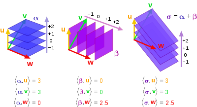
Visualizing linear functionals

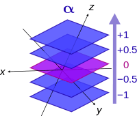
Geometric interpretation of a 1-form α as a stack of hyperplanes of constant value, each corresponding to those vectors that α maps to a given scalar value shown next to it along with the "sense" of increase. The zero plane is through the origin.

In finite dimensions, a linear functional can be visualized in terms of its level sets, the sets of vectors which map to a given value. In three dimensions, the level sets of a linear functional are a family of mutually parallel planes; in higher dimensions, they are parallel hyperplanes. This method of visualizing linear functionals is sometimes introduced in general relativity texts, such as Gravitation by Misner, Thorne & Wheeler (1973).

Dual vectors and bilinear forms

Linear functionals (1-forms) α, β and their sum σ and vectors u, v, w, in 3d Euclidean space. The number of (1-form) hyperplanes intersected by a vector equals the inner product.[15]

Every non-degenerate bilinear form on a finite-dimensional vector space V induces an isomorphism V → V^∗ : v ↦ v^∗ such that

v^{*}(w):=\langle v,w\rangle \quad \forall w\in V,

where the bilinear form on V is denoted ⟨ , ⟩ (for instance, in Euclidean space ⟨v, w⟩ = v ⋅ w is the dot product of v and w).

The inverse isomorphism is V^∗ → V : v^∗ ↦ v, where v is the unique element of V such that

\langle v,w\rangle =v^{*}(w)\quad \forall w\in V.

The above defined vector v^∗ ∈ V^∗ is said to be the dual vector of v ∈ V.

In an infinite dimensional Hilbert space, analogous results hold by the Riesz representation theorem. There is a mapping V → V^∗ into the continuous dual space V^∗. However, this mapping is antilinear rather than linear.

Bases in finite dimensions

Basis of the dual space in finite dimensions

Let the vector space V have a basis ${\vec {e}}_{1},{\vec {e}}_{2},\dots ,{\vec {e}}_{n}$ , not necessarily orthogonal. Then the dual space V* has a basis ${\tilde {\omega }}^{1},{\tilde {\omega }}^{2},\dots ,{\tilde {\omega }}^{n}$ called the dual basis defined by the special property that

{\tilde {\omega }}^{i}({\vec {e}}_{j})=\left\{{\begin{matrix}1&\mathrm {if} \ i=j\\0&\mathrm {if} \ i\not =j.\end{matrix}}\right.

Or, more succinctly,

{\tilde {\omega }}^{i}({\vec {e}}_{j})=\delta _{ij}

where δ is the Kronecker delta. Here the superscripts of the basis functionals are not exponents but are instead contravariant indices.

A linear functional ${\tilde {u}}$ belonging to the dual space ${\tilde {V}}$ can be expressed as a linear combination of basis functionals, with coefficients ("components") u_i,

{\tilde {u}}=\sum _{i=1}^{n}u_{i}\,{\tilde {\omega }}^{i}.

Then, applying the functional ${\tilde {u}}$ to a basis vector e_j yields

{\tilde {u}}({\vec {e}}_{j})=\sum _{i=1}^{n}\left(u_{i}\,{\tilde {\omega }}^{i}\right){\vec {e}}_{j}=\sum _{i}u_{i}\left[{\tilde {\omega }}^{i}\left({\vec {e}}_{j}\right)\right]

due to linearity of scalar multiples of functionals and pointwise linearity of sums of functionals. Then

{\begin{aligned}{\tilde {u}}({\vec {e}}_{j})&=\sum _{i}u_{i}\left[{\tilde {\omega }}^{i}\left({\vec {e}}_{j}\right)\right]=\sum _{i}u_{i}{\delta ^{i}}_{j}\\&=u_{j}.\end{aligned}}

So each component of a linear functional can be extracted by applying the functional to the corresponding basis vector.

The dual basis and inner product

When the space V carries an inner product, then it is possible to write explicitly a formula for the dual basis of a given basis. Let V have (not necessarily orthogonal) basis ${\vec {e}}_{1},\dots ,{\vec {e}}_{n}$ . In three dimensions (n = 3), the dual basis can be written explicitly

{\tilde {\omega }}^{i}({\vec {v}})={1 \over 2}\,\left\langle {\sum _{j=1}^{3}\sum _{k=1}^{3}\varepsilon ^{ijk}\,({\vec {e}}_{j}\times {\vec {e}}_{k}) \over {\vec {e}}_{1}\cdot {\vec {e}}_{2}\times {\vec {e}}_{3}},{\vec {v}}\right\rangle ,

for i = 1, 2, 3, where ε is the Levi-Civita symbol and $\langle ,\rangle$ the inner product (or dot product) on V.

In higher dimensions, this generalizes as follows

{\tilde {\omega }}^{i}({\vec {v}})=\left\langle {\frac {{\underset {{}^{1\leq i_{2}<i_{3}<\dots <i_{n}\leq n}}{\sum }}\varepsilon ^{ii_{2}\dots i_{n}}(\star {\vec {e}}_{i_{2}}\wedge \dots \wedge {\vec {e}}_{i_{n}})}{\star ({\vec {e}}_{1}\wedge \dots \wedge {\vec {e}}_{n})}},{\vec {v}}\right\rangle ,

where $\star$ is the Hodge star operator.

Notes

This follows since just as the image of a vector subspace under a linear transformation is a vector subspace, so is the image of $X$ under $f$ . However, the only vector subspaces (that is, $𝕂$ -subspaces) of $𝕂$ are ${ 0$ } and $𝕂$ itself.
If $g \in X ℝ #$ is non-trivial then the range of $g$ is $ℝ$ ; but then g can't belong to $X #$ because if it did, then its range would have to be $ℂ$ rather than $ℝ$ .
Narici 2011, pp. 177-220.
Narici 2011, pp. 10-11.
Obvious if $X$ is a real vector space. For the non-trivial direction, assume that $Re f \leq p$ on $X$ and let $x \in X$ . Let $r \geq 0$ and $t$ be real numbers such that $f (x) = re it$ . Then $| f (x) | = r = f (e - it x) = Re (f (e - it x)) \leq p (e - it x) = p (x)$ .
Wilansky 2013, p. 20.
Narici 2011, p. 128.
Narici 2011, p. 126.
Rudin 1991, pp. 63-64.
Narici 2011, pp. 1-18.
Rudin 1991, Theorem 1.18
Narici 2011, pp. 225-273.
Schaefer, Corollary 4.3
Lax 1996
J.A. Wheeler; C. Misner; K.S. Thorne (1973). Gravitation. W.H. Freeman & Co. p. 57. ISBN 0-7167-0344-0.

References

Bishop, Richard; Goldberg, Samuel (1980), "Chapter 4", Tensor Analysis on Manifolds, Dover Publications, ISBN 0-486-64039-6
Conway, John B. (1990). A Course in Functional Analysis. Graduate Texts in Mathematics. 96 (2nd ed.). Springer. ISBN 0-387-97245-5.
Dunford, Nelson (1988). Linear operators (in Romanian). New York: Interscience Publishers. ISBN 0-471-60848-3. OCLC 18412261.
Halmos, Paul (1974), Finite dimensional vector spaces, Springer, ISBN 0-387-90093-4
Lax, Peter (1996), Linear algebra, Wiley-Interscience, ISBN 978-0-471-11111-5
Misner, Charles W.; Thorne, Kip. S.; Wheeler, John A. (1973), Gravitation, W. H. Freeman, ISBN 0-7167-0344-0
Narici, Lawrence; Beckenstein, Edward (2011). Topological Vector Spaces. Pure and applied mathematics (Second ed.). Boca Raton, FL: CRC Press. ISBN 978-1584888666. OCLC 144216834.
Rudin, Walter (January 1, 1991). Functional Analysis. International Series in Pure and Applied Mathematics. 8 (Second ed.). New York, NY: McGraw-Hill Science/Engineering/Math. ISBN 978-0-07-054236-5. OCLC 21163277.CS1 maint: ref=harv (link) CS1 maint: date and year (link)
Schaefer, Helmut H.; Wolff, Manfred P. (1999). Topological Vector Spaces. GTM. 8 (Second ed.). New York, NY: Springer New York Imprint Springer. ISBN 978-1-4612-7155-0. OCLC 840278135.CS1 maint: ref=harv (link)
Schutz, Bernard (1985), "Chapter 3", A first course in general relativity, Cambridge, UK: Cambridge University Press, ISBN 0-521-27703-5
Trèves, François (August 6, 2006) [1967]. Topological Vector Spaces, Distributions and Kernels. Mineola, N.Y.: Dover Publications. ISBN 978-0-486-45352-1. OCLC 853623322.CS1 maint: ref=harv (link) CS1 maint: date and year (link)

This article is issued from Wikipedia. The text is licensed under Creative Commons - Attribution - Sharealike. Additional terms may apply for the media files.

[1] This follows since just as the image of a vector subspace under a linear transformation is a vector subspace, so is the image of $X$ under $f$ . However, the only vector subspaces (that is, $𝕂$ -subspaces) of $𝕂$ are ${ 0$ } and $𝕂$ itself.

[2] If $g \in X ℝ #$ is non-trivial then the range of $g$ is $ℝ$ ; but then g can't belong to $X #$ because if it did, then its range would have to be $ℂ$ rather than $ℝ$ .

[FOOTNOTENarici2011177-220-3] Narici 2011, pp. 177-220.

[FOOTNOTENarici201110-11-4] Narici 2011, pp. 10-11.

[5] Obvious if $X$ is a real vector space. For the non-trivial direction, assume that $Re f \leq p$ on $X$ and let $x \in X$ . Let $r \geq 0$ and $t$ be real numbers such that $f (x) = re it$ . Then $| f (x) | = r = f (e - it x) = Re (f (e - it x)) \leq p (e - it x) = p (x)$ .

[FOOTNOTEWilansky201320-6] Wilansky 2013, p. 20.

[FOOTNOTENarici2011128-7] Narici 2011, p. 128.

[FOOTNOTENarici2011126-8] Narici 2011, p. 126.

[FOOTNOTERudin199163-64-9] Rudin 1991, pp. 63-64.

[FOOTNOTENarici20111-18-10] Narici 2011, pp. 1-18.

[11] Rudin 1991, Theorem 1.18

[FOOTNOTENarici2011225-273-12] Narici 2011, pp. 225-273.

[13] Schaefer, Corollary 4.3

[14] Lax 1996

[15] J.A. Wheeler; C. Misner; K.S. Thorne (1973). Gravitation. W.H. Freeman & Co. p. 57. ISBN 0-7167-0344-0.

Functional analysis (topics, glossary)
Spaces	Hilbert space, Banach space, Fréchet space, topological vector space
Theorems	Hahn–Banach theorem, closed graph theorem, uniform boundedness principle, Kakutani fixed-point theorem, Krein–Milman theorem, min-max theorem, Gelfand–Naimark theorem, Banach–Alaoglu theorem
Operators	bounded operator, compact operator, adjoint operator, unitary operator, Hilbert–Schmidt operator, trace class, unbounded operator
Algebras	Banach algebra, C-algebra, spectrum of a C-algebra, operator algebra, group algebra of a locally compact group, von Neumann algebra
Open problems	invariant subspace problem, Mahler's conjecture
Applications	Besov space, Hardy space, spectral theory of ordinary differential equations, heat kernel, index theorem, calculus of variation, functional calculus, integral operator, Jones polynomial, topological quantum field theory, noncommutative geometry, Riemann hypothesis
Advanced topics	locally convex space, approximation property, balanced set, Schwartz space, weak topology, barrelled space, Banach–Mazur distance, Tomita–Takesaki theory

Topological vector spaces (TVSs)
Basic concepts	Banach space Continuous linear operator Functionals Hilbert space Linear operators Locally convex space Homomorphism Topological vector space Vector space
Main results	Closed graph theorem F. Riesz's theorem Hahn–Banach (hyperplane separation Vector-Valued Hahn-Banach) Open mapping (Banach–Schauder) (Bounded inverse) Uniform boundedness (Banach–Steinhaus)
Maps	Almost open Bilinear (form operator) and Sesquilinear forms Closed Compact operator Continuous and Discontinuous Linear maps Densely defined Homomorphism Functionals Norm Operator Seminorm Sublinear Transpose
Types of sets	Absolutely convex/disk Absorbing/Radial Affine Balanced/Circled Bounding points Bounded Complemented subspace Convex Convex cone (subset) Linear cone (subset) Extreme point Pre-compact/Totally bounded Radial Radially convex/Star-shaped Symmetric
Set operations	Affine hull (Relative) Algebraic interior (core) Convex hull Linear span Minkowski addition Polar (Quasi) Relative interior
Types of TVSs	Asplund B-complete/Ptak Banach (Countably) Barrelled (Ultra-) Bornological Brauner Complete (DF)-space Distinguished F-space Fréchet (tame Fréchet) Grothendieck Hilbert Infrabarreled Interpolation space LB-space LF-space Locally convex space Mackey (Pseudo)Metrizable Montel Quasibarrelled Quasi-complete Quasinormed (Polynomially Semi-) Reflexive Riesz Schwartz Semi-complete Smith Stereotype (B Strictly Uniformly convex (Quasi-) Ultrabarrelled Uniformly smooth Webbed With the Approximation property

Linear form

Linear functionals on real or complex vector spaces

Basic definitions

Relationships with other maps

Relationship between real and complex linear functionals

Relationships with seminorms and sublinear functions

Hahn-Banach theorem

Relationships between multiple linear functionals

Hyperplanes and maximal subspaces

Continuous linear functionals

Equicontinuity of families of linear functionals

Examples and applications

Linear functionals in Rn

(Definite) Integration

Evaluation

Application to quadrature

Linear functionals in quantum mechanics

Distributions

Visualizing linear functionals

Dual vectors and bilinear forms

Bases in finite dimensions

Basis of the dual space in finite dimensions

The dual basis and inner product

See also

Notes

References

Linear functionals in Rⁿ