Skewness

In probability theory and statistics, skewness is a measure of the asymmetry of the probability distribution of a real-valued random variable about its mean. The skewness value can be positive, zero, negative, or undefined.

Example distribution with non-zero (positive) skewness. These data are from experiments on wheat grass growth.

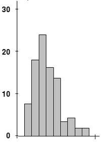
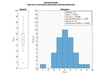
For a unimodal distribution, negative skew commonly indicates that the tail is on the left side of the distribution, and positive skew indicates that the tail is on the right. In cases where one tail is long but the other tail is fat, skewness does not obey a simple rule. For example, a zero value means that the tails on both sides of the mean balance out overall; this is the case for a symmetric distribution, but can also be true for an asymmetric distribution where one tail is long and thin, and the other is short but fat.

Introduction

Consider the two distributions in the figure just below. Within each graph, the values on the right side of the distribution taper differently from the values on the left side. These tapering sides are called tails, and they provide a visual means to determine which of the two kinds of skewness a distribution has:

1. negative skew: The left tail is longer; the mass of the distribution is concentrated on the right of the figure. The distribution is said to be left-skewed, left-tailed, or skewed to the left, despite the fact that the curve itself appears to be skewed or leaning to the right; left instead refers to the left tail being drawn out and, often, the mean being skewed to the left of a typical center of the data. A left-skewed distribution usually appears as a right-leaning curve.[1]
2. positive skew: The right tail is longer; the mass of the distribution is concentrated on the left of the figure. The distribution is said to be right-skewed, right-tailed, or skewed to the right, despite the fact that the curve itself appears to be skewed or leaning to the left; right instead refers to the right tail being drawn out and, often, the mean being skewed to the right of a typical center of the data. A right-skewed distribution usually appears as a left-leaning curve.[1]

Skewness in a data series may sometimes be observed not only graphically but by simple inspection of the values. For instance, consider the numeric sequence (49, 50, 51), whose values are evenly distributed around a central value of 50. We can transform this sequence into a negatively skewed distribution by adding a value far below the mean, which is probably a negative outlier, e.g. (40, 49, 50, 51). Therefore, the mean of the sequence becomes 47.5, and the median is 49.5. Based on the formula of nonparametric skew, defined as ${\displaystyle (\mu -\nu )/\sigma ,}$ the skew is negative. Similarly, we can make the sequence positively skewed by adding a value far above the mean, which is probably a positive outlier, e.g. (49, 50, 51, 60), where the mean is 52.5, and the median is 50.5.

As mentioned earlier, a unimodal distribution with zero value of skewness does not imply that this distribution is symmetric necessarily. However, a symmetric unimodal or multimodal distribution always has zero skewness.

Example of an asymmetric distribution with zero skewness. This figure serves as a counterexample that zero skewness does not imply symmetric distribution necessarily. (Skewness was calculated by Pearson's moment coefficient of skewness.)

Relationship of mean and median

The skewness is not directly related to the relationship between the mean and median: a distribution with negative skew can have its mean greater than or less than the median, and likewise for positive skew.[2]

A general relationship of mean and median under differently skewed unimodal distribution

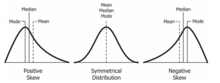
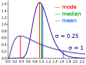
In the older notion of nonparametric skew, defined as ${\displaystyle (\mu -\nu )/\sigma ,}$ where ${\displaystyle \mu }$ is the mean, ${\displaystyle \nu }$ is the median, and ${\displaystyle \sigma }$ is the standard deviation, the skewness is defined in terms of this relationship: positive/right nonparametric skew means the mean is greater than (to the right of) the median, while negative/left nonparametric skew means the mean is less than (to the left of) the median. However, the modern definition of skewness and the traditional nonparametric definition do not always have the same sign: while they agree for some families of distributions, they differ in some of the cases, and conflating them is misleading.

If the distribution is symmetric, then the mean is equal to the median, and the distribution has zero skewness.[3] If the distribution is both symmetric and unimodal, then the mean = median = mode. This is the case of a coin toss or the series 1,2,3,4,... Note, however, that the converse is not true in general, i.e. zero skewness does not imply that the mean is equal to the median.

A 2005 journal article points out:[2]

Many textbooks teach a rule of thumb stating that the mean is right of the median under right skew, and left of the median under left skew. This rule fails with surprising frequency. It can fail in multimodal distributions, or in distributions where one tail is long but the other is heavy. Most commonly, though, the rule fails in discrete distributions where the areas to the left and right of the median are not equal. Such distributions not only contradict the textbook relationship between mean, median, and skew, they also contradict the textbook interpretation of the median.

Distribution of adult residents across US households

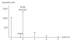
For example, in the distribution of adult residents across US households, the skew is to the right. However, due to the majority of cases is less or equal to the mode, which is also the median, the mean sits in the heavier left tail. As a result, the rule of thumb that the mean is right of the median under right skew failed.[2]

Definition

Pearson's moment coefficient of skewness

The skewness of a random variable X is the third standardized moment ${\displaystyle {\tilde {\mu }}_{3}}$, defined as:[4][5]

${\displaystyle {\tilde {\mu }}_{3}=\operatorname {E} \left[\left({\frac {X-\mu }{\sigma }}\right)^{3}\right]={\frac {\mu _{3}}{\sigma ^{3}}}={\frac {\operatorname {E} \left[(X-\mu )^{3}\right]}{(\operatorname {E} \left[(X-\mu )^{2}\right])^{3/2}}}={\frac {\kappa _{3}}{\kappa _{2}^{3/2}}}}$

where μ is the mean, σ is the standard deviation, E is the expectation operator, μ₃ is the third central moment, and κ_t are the t-th cumulants. It is sometimes referred to as Pearson's moment coefficient of skewness,[5] or simply the moment coefficient of skewness,[4] but should not be confused with Pearson's other skewness statistics (see below). The last equality expresses skewness in terms of the ratio of the third cumulant κ₃ to the 1.5th power of the second cumulant κ₂. This is analogous to the definition of kurtosis as the fourth cumulant normalized by the square of the second cumulant. The skewness is also sometimes denoted Skew[X].

If σ is finite, μ is finite too and skewness can be expressed in terms of the non-central moment E[X³] by expanding the previous formula,

${\displaystyle {\begin{aligned}{\tilde {\mu }}_{3}&=\operatorname {E} \left[\left({\frac {X-\mu }{\sigma }}\right)^{3}\right]\\&={\frac {\operatorname {E} [X^{3}]-3\mu \operatorname {E} [X^{2}]+3\mu ^{2}\operatorname {E} [X]-\mu ^{3}}{\sigma ^{3}}}\\&={\frac {\operatorname {E} [X^{3}]-3\mu (\operatorname {E} [X^{2}]-\mu \operatorname {E} [X])-\mu ^{3}}{\sigma ^{3}}}\\&={\frac {\operatorname {E} [X^{3}]-3\mu \sigma ^{2}-\mu ^{3}}{\sigma ^{3}}}.\end{aligned}}}$

Examples

Skewness can be infinite, as when

${\displaystyle \Pr \left[X>x\right]=x^{-2}{\mbox{ for }}x>1,\ \Pr[X<1]=0}$

where the third cumulants are infinite, or as when

${\displaystyle \Pr[X<x]=(1-x)^{-3}/2{\mbox{ for negative }}x{\mbox{ and }}\Pr[X>x]=(1+x)^{-3}/2{\mbox{ for positive }}x.}$

where the third cumulant is undefined.

Examples of distributions with finite skewness include the following.

• A normal distribution and any other symmetric distribution with finite third moment has a skewness of 0
• A half-normal distribution has a skewness just below 1
• An exponential distribution has a skewness of 2
• A lognormal distribution can have a skewness of any positive value, depending on its parameters

Sample skewness

For a sample of n values, a natural method of moments estimator of the population skewness is[6]

${\displaystyle b_{1}={\frac {m_{3}}{s^{3}}}={\frac {{\tfrac {1}{n}}\sum _{i=1}^{n}(x_{i}-{\overline {x}})^{3}}{{\sqrt {{\tfrac {1}{n-1}}\sum _{i=1}^{n}(x_{i}-{\overline {x}})^{2}}}^{\,3}}}={\frac {{\tfrac {1}{n}}\sum _{i=1}^{n}(x_{i}-{\overline {x}})^{3}}{\left[{\tfrac {1}{n-1}}\sum _{i=1}^{n}(x_{i}-{\overline {x}})^{2}\right]^{3/2}}},}$

where ${\displaystyle {\overline {x}}}$ is the sample mean, s is the sample standard deviation, and the numerator m₃ is the sample third central moment. This formula can be thought of as the average cubed deviation in the sample divided by the cubed sample standard deviation.

Another common definition of the sample skewness is[6][7]

${\displaystyle {\begin{aligned}G_{1}&={\frac {k_{3}}{k_{2}^{3/2}}}={\frac {n^{2}}{(n-1)(n-2)}}\;{\frac {m_{3}}{s^{3}}}\\&={\frac {\sqrt {n(n-1)}}{n-2}}{\frac {m_{3}}{m_{2}^{3/2}}}={\frac {\sqrt {n(n-1)}}{n-2}}\left[{\frac {{\frac {1}{n}}\sum \limits _{i=1}^{n}{(x_{i}-{\bar {x}})}^{3}}{\left({\frac {1}{n}}\sum \limits _{i=1}^{n}(x_{i}-{\bar {x}})^{2}\right)^{3/2}}}\right],\\\end{aligned}}}$

where ${\displaystyle k_{3}}$ is the unique symmetric unbiased estimator of the third cumulant and ${\displaystyle k_{2}=s^{2}}$ is the symmetric unbiased estimator of the second cumulant (i.e. the variance).

In general, the ratios ${\displaystyle b_{1}}$ and ${\displaystyle G_{1}}$ are both biased estimators of the population skewness ${\displaystyle \gamma _{1}}$; their expected values can even have the opposite sign from the true skewness. (For instance, a mixed distribution consisting of very thin Gaussians centred at −99, 0.5, and 2 with weights 0.01, 0.66, and 0.33 has a skewness of about −9.77, but in a sample of 3, ${\displaystyle G_{1}}$ has an expected value of about 0.32, since usually all three samples are in the positive-valued part of the distribution, which is skewed the other way.) Nevertheless, ${\displaystyle b_{1}}$ and ${\displaystyle G_{1}}$ each have obviously the correct expected value of zero for any symmetric distribution with a finite third moment, including a normal distribution.

Under the assumption that the underlying random variable ${\displaystyle X}$ is normally distributed, it can be shown that ${\displaystyle {\sqrt {n}}b_{1}{\xrightarrow {d}}N(0,6)}$, i.e., its distribution converges to a normal distribution with mean 0 and variance 6. The variance of the skewness of a random sample of size n from a normal distribution is[8][9]

${\displaystyle \operatorname {var} (G_{1})={\frac {6n(n-1)}{(n-2)(n+1)(n+3)}}.}$

An approximate alternative is 6/n, but this is inaccurate for small samples.

In normal samples, ${\displaystyle b_{1}}$ has the smaller variance of the two estimators, with

${\displaystyle \operatorname {var} (b_{1})<\operatorname {var} \left({\frac {m_{3}}{m_{2}^{3/2}}}\right)<\operatorname {var} (G_{1}),}$

where m₂ in the denominator is the (biased) sample second central moment.[6]

The adjusted Fisher–Pearson standardized moment coefficient ${\displaystyle G_{1}}$ is the version found in Excel and several statistical packages including Minitab, SAS and SPSS.[10]

Applications

Skewness is a descriptive statistic that can be used in conjunction with the histogram and the normal quantile plot to characterize the data or distribution.

Skewness indicates the direction and relative magnitude of a distribution's deviation from the normal distribution.

With pronounced skewness, standard statistical inference procedures such as a confidence interval for a mean will be not only incorrect, in the sense that the true coverage level will differ from the nominal (e.g., 95%) level, but they will also result in unequal error probabilities on each side.

Skewness can be used to obtain approximate probabilities and quantiles of distributions (such as value at risk in finance) via the Cornish-Fisher expansion.

Many models assume normal distribution; i.e., data are symmetric about the mean. The normal distribution has a skewness of zero. But in reality, data points may not be perfectly symmetric. So, an understanding of the skewness of the dataset indicates whether deviations from the mean are going to be positive or negative.

D'Agostino's K-squared test is a goodness-of-fit normality test based on sample skewness and sample kurtosis.

Other measures of skewness

Comparison of mean, median and mode of two log-normal distributions with the same medians and different skewnesses.

Other measures of skewness have been used, including simpler calculations suggested by Karl Pearson[11] (not to be confused with Pearson's moment coefficient of skewness, see above). These other measures are:

Pearson's first skewness coefficient (mode skewness)

The Pearson mode skewness,[12] or first skewness coefficient, is defined as

mean − mode/standard deviation.

Pearson's second skewness coefficient (median skewness)

The Pearson median skewness, or second skewness coefficient,[13][14] is defined as

3 (mean − median)/standard deviation.

Which is a simple multiple of the nonparametric skew.

Quantile-based measures

Bowley's measure of skewness (from 1901),[15][16] also called Yule's coefficient (from 1912)[17][18] is defined as:

${\displaystyle B_{1}={\frac {{{Q}_{3}}+{{Q}_{1}}-2{{Q}_{2}}}{{{Q}_{3}}-{{Q}_{1}}}}}$.

When writing it as ${\displaystyle {\frac {{\frac {{{Q}_{3}}+{{Q}_{1}}}{2}}-{{Q}_{2}}}{\frac {{{Q}_{3}}-{{Q}_{1}}}{2}}}}$, it is easier to see that the numerator is difference between the average of the upper and lower quartiles (a measure of location) and the median (another measure of location), while the denominator is the semi-interquartile range (Q3-Q1)/2, which for symmetric distributions is the MAD measure of dispersion.

Other names for this measure are Galton's measure of skewness,[19] the Yule–Kendall index[20] and the quartile skewness[21] ,

A more general formulation of a skewness function was described by Groeneveld, R. A. and Meeden, G. (1984):[22][23][24]

${\displaystyle \gamma (u)={\frac {F^{-1}(u)+F^{-1}(1-u)-2F^{-1}(1/2)}{F^{-1}(u)-F^{-1}(1-u)}}}$

where F is the cumulative distribution function. This leads to a corresponding overall measure of skewness[23] defined as the supremum of this over the range 1/2 ≤ u < 1. Another measure can be obtained by integrating the numerator and denominator of this expression.[22] The function γ(u) satisfies −1 ≤ γ(u) ≤ 1 and is well defined without requiring the existence of any moments of the distribution.[22] Quantile-based skewness measures are at first glance easy to interpret, but they often show significantly larger sample variations, than moment-based methods. This means that often samples from a symmetric distribution (like the uniform distribution) have a large quantile-based skewness, just by chance.

Bowley's measure of skewness is γ(u) evaluated at u = 3/4. Kelley's measure of skewness uses u = 0.1.[25]

Groeneveld & Meeden’s coefficient

Groeneveld & Meeden have suggested, as an alternative measure of skewness,[22]

${\displaystyle B_{3}=\mathrm {skew} (X)={\frac {(\mu -\nu )}{E(|X-\nu |)}},}$

where μ is the mean, ν is the median, |...| is the absolute value, and E() is the expectation operator. This is closely related in form to Pearson's second skewness coefficient.

L-moments

Use of L-moments in place of moments provides a measure of skewness known as the L-skewness.[26]

Distance skewness

A value of skewness equal to zero does not imply that the probability distribution is symmetric. Thus there is a need for another measure of asymmetry that has this property: such a measure was introduced in 2000.[27] It is called distance skewness and denoted by dSkew. If X is a random variable taking values in the d-dimensional Euclidean space, X has finite expectation, X' is an independent identically distributed copy of X, and ${\displaystyle \|\cdot \|}$ denotes the norm in the Euclidean space, then a simple measure of asymmetry with respect to location parameter θ is

${\displaystyle \operatorname {dSkew} (X):=1-{\frac {\operatorname {E} \|X-X'\|}{\operatorname {E} \|X+X'-2\theta \|}}{\text{ if }}\Pr(X=\theta )\neq 1}$

and dSkew(X) := 0 for X = θ (with probability 1). Distance skewness is always between 0 and 1, equals 0 if and only if X is diagonally symmetric with respect to θ (X and 2θ−X have the same probability distribution) and equals 1 if and only if X is a constant c (${\displaystyle c\neq \theta }$) with probability one.[28] Thus there is a simple consistent statistical test of diagonal symmetry based on the sample distance skewness:

${\displaystyle \operatorname {dSkew} _{n}(X):=1-{\frac {\sum _{i,j}\|x_{i}-x_{j}\|}{\sum _{i,j}\|x_{i}+x_{j}-2\theta \|}}.}$

Medcouple

The medcouple is a scale-invariant robust measure of skewness, with a breakdown point of 25%.[29] It is the median of the values of the kernel function

${\displaystyle h(x_{i},x_{j})={\frac {(x_{i}-x_{m})-(x_{m}-x_{j})}{x_{i}-x_{j}}}}$

taken over all couples ${\displaystyle (x_{i},x_{j})}$ such that ${\displaystyle x_{i}\geq x_{m}\geq x_{j}}$, where ${\displaystyle x_{m}}$ is the median of the sample ${\displaystyle \{x_{1},x_{2},\ldots ,x_{n}\}}$. It can be seen as the median of all possible quantile skewness measures.

See also

• Bragg peak
• Coskewness
• Kurtosis
• Shape parameters
• Skew normal distribution
• Skewness risk

References

Citations

1. Susan Dean, Barbara Illowsky "Descriptive Statistics: Skewness and the Mean, Median, and Mode", Connexions website
2. von Hippel, Paul T. (2005). "Mean, Median, and Skew: Correcting a Textbook Rule". Journal of Statistics Education. 13 (2).
3. "1.3.5.11. Measures of Skewness and Kurtosis". NIST. Retrieved 18 March 2012.
4. "Measures of Shape: Skewness and Kurtosis", 2008–2016 by Stan Brown, Oak Road Systems
5. Pearson's moment coefficient of skewness, FXSolver.com
6. Joanes, D. N.; Gill, C. A. (1998). "Comparing measures of sample skewness and kurtosis". Journal of the Royal Statistical Society, Series D. 47 (1): 183–189. doi:10.1111/1467-9884.00122.
7. Doane, David P., and Lori E. Seward. "Measuring skewness: a forgotten statistic." Journal of Statistics Education 19.2 (2011): 1-18. (Page 7)
8. Duncan Cramer (1997) Fundamental Statistics for Social Research. Routledge. ISBN 9780415172042 (p 85)
9. Kendall, M.G.; Stuart, A. (1969) The Advanced Theory of Statistics, Volume 1: Distribution Theory, 3rd Edition, Griffin. ISBN 0-85264-141-9 (Ex 12.9)
10. Doane DP, Seward LE (2011) J Stat Educ 19 (2)
11. "Archived copy" (PDF). Archived from the original (PDF) on 5 July 2010. Retrieved 9 April 2010.CS1 maint: archived copy as title (link)
12. Weisstein, Eric W. "Pearson Mode Skewness". MathWorld.
13. Weisstein, Eric W. "Pearson's skewness coefficients". MathWorld.
14. Doane, David P.; Seward, Lori E. (2011). "Measuring Skewness: A Forgotten Statistic?" (PDF). Journal of Statistics Education. 19 (2): 1–18. doi:10.1080/10691898.2011.11889611.
15. Bowley, A. L. (1901). Elements of Statistics, P.S. King & Son, Laondon. Or in a later edition: BOWLEY, AL. "Elements of Statistics, 4th Edn (New York, Charles Scribner)."(1920).
16. Kenney JF and Keeping ES (1962) Mathematics of Statistics, Pt. 1, 3rd ed., Van Nostrand, (page 102).
17. Yule, George Udny. An introduction to the theory of statistics. C. Griffin, limited, 1912.
18. Groeneveld, Richard A (1991). "An influence function approach to describing the skewness of a distribution". The American Statistician. 45 (2): 97–102. doi:10.2307/2684367. JSTOR 2684367.
19. Johnson et al (1994) p 3, p 40
20. Wilks DS (1995) Statistical Methods in the Atmospheric Sciences, p 27. Academic Press. ISBN 0-12-751965-3
21. Weisstein, Eric W. "Skewness". mathworld.wolfram.com. Retrieved 21 November 2019.
22. Groeneveld, R.A.; Meeden, G. (1984). "Measuring Skewness and Kurtosis". The Statistician. 33 (4): 391–399. doi:10.2307/2987742. JSTOR 2987742.
23. MacGillivray (1992)
24. Hinkley DV (1975) "On power transformations to symmetry", Biometrika, 62, 101–111
25. A.W.L. Pubudu Thilan. "Applied Statistics I: Chapter 5: Measures of skewness" (PDF). University of Ruhuna. p. 21.
26. Hosking, J.R.M. (1992). "Moments or L moments? An example comparing two measures of distributional shape". The American Statistician. 46 (3): 186–189. doi:10.2307/2685210. JSTOR 2685210.
27. Szekely, G.J. (2000). "Pre-limit and post-limit theorems for statistics", In: Statistics for the 21st Century (eds. C. R. Rao and G. J. Szekely), Dekker, New York, pp. 411–422.
28. Szekely, G. J. and Mori, T. F. (2001) "A characteristic measure of asymmetry and its application for testing diagonal symmetry", Communications in Statistics – Theory and Methods 30/8&9, 1633–1639.
29. G. Brys; M. Hubert; A. Struyf (November 2004). "A Robust Measure of Skewness". Journal of Computational and Graphical Statistics. 13 (4): 996–1017. doi:10.1198/106186004X12632.

Sources

• Johnson, NL, Kotz, S, Balakrishnan N (1994) Continuous Univariate Distributions, Vol 1, 2nd Edition Wiley. ISBN 0-471-58495-9.
• MacGillivray, HL (1992). "Shape properties of the g- and h- and Johnson families". Communications in Statistics - Theory and Methods. 21 (5): 1244–1250. doi:10.1080/03610929208830842.
• Premaratne, G., Bera, A. K. (2001). Adjusting the Tests for Skewness and Kurtosis for Distributional Misspecifications. Working Paper Number 01-0116, University of Illinois. Forthcoming in Comm in Statistics, Simulation and Computation. 2016 1-15
• Premaratne, G., Bera, A. K. (2000). Modeling Asymmetry and Excess Kurtosis in Stock Return Data. Office of Research Working Paper Number 00-0123, University of Illinois.
• Skewness Measures for the Weibull Distribution

External links

• "Asymmetry coefficient", Encyclopedia of Mathematics, EMS Press, 2001 [1994]
• An Asymmetry Coefficient for Multivariate Distributions by Michel Petitjean
• On More Robust Estimation of Skewness and Kurtosis Comparison of skew estimators by Kim and White.
• Closed-skew Distributions — Simulation, Inversion and Parameter Estimation