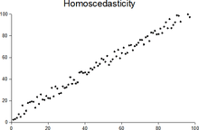
Homoscedasticity
In statistics, a sequence (or a vector) of random variables is homoscedastic /ˌhoʊmoʊskəˈdæstɪk/ if all its random variables have the same finite variance. This is also known as homogeneity of variance. The complementary notion is called heteroscedasticity. The spellings homoskedasticity and heteroskedasticity are also frequently used.[1]

Assuming a variable is homoscedastic when in reality it is heteroscedastic /ˌhɛtəroʊskəˈdæstɪk/) results in unbiased but inefficient point estimates and in biased estimates of standard errors, and may result in overestimating the goodness of fit as measured by the Pearson coefficient.
Assumptions of a regression model
A standard assumption in a linear regression, is that the variance of the disturbance term is the same across observations, and in particular does not depend on the values of the explanatory variables [2] This is one of the assumptions under which the Gauss–Markov theorem applies and ordinary least squares (OLS) gives the best linear unbiased estimator ("BLUE"). Homoscedasticity is not required for the coefficient estimates to be unbiased, consistent, and asymptotically normal, but it is required for OLS to be efficient.[3] It is also required for the standard errors of the estimates to be unbiased and consistent, so it is required for accurate hypothesis testing, e.g. for a t-test of whether a coefficient is significantly different from zero.
A more formal way to state the assumption of homoskedasticity is that the diagonals of the variance-covariance matrix of must all be the same number: , where is the same for all i.[4] Note that this still allows for the off-diagonals, the covariances , to be nonzero, which is a separate violation of the Gauss-Markov assumptions known as serial correlation.
Examples
The matrices below are covariances of the disturbance, with entries , when there are just three observations across time. The disturbance in matrix A is homoskedastic; this is the simple case where OLS is the best linear unbiased estimator. The disturbances in matrices B and C are heteroskedastic. In matrix B, the variance is time-varying, increasing steadily across time; in matrix C, the variance depends on the value of x. The disturbance in matrix D is homoskedastic because the diagonal variances are constant, even though the off-diagonal covariances are non-zero and ordinary least squares is inefficient for a different reason: serial correlation.
If y is consumption, x is income, and is whims of the consumer, and we are estimating then if richer consumers' whims affect their spending more in absolute dollars, we might have rising with income, as in matrix C above.[5]
Testing
Residuals can be tested for homoscedasticity using the Breusch–Pagan test, which performs an auxiliary regression of the squared residuals on the independent variables. From this auxiliary regression, the explained sum of squares is retained, divided by two, and then becomes the test statistic for a chi-squared distribution with the degrees of freedom equal to the number of independent variables. The null hypothesis of this chi-squared test is homoscedasticity, and the alternative hypothesis would indicate heteroscedasticity. Since the Breusch–Pagan test is sensitive to departures from normality or small sample sizes, the Koenker–Bassett or 'generalized Breusch–Pagan' test is commonly used instead. From the auxiliary regression, it retains the R-squared value which is then multiplied by the sample size, and then becomes the test statistic for a chi-squared distribution (and uses the same degrees of freedom). Although it is not necessary for the Koenker–Bassett test, the Breusch–Pagan test requires that the squared residuals also be divided by the residual sum of squares divided by the sample size.[6] Testing for groupwise heteroscedasticity requires the Goldfeld–Quandt test.
Homoscedastic distributions
Two or more normal distributions, , are homoscedastic if they share a common covariance (or correlation) matrix, . Homoscedastic distributions are especially useful to derive statistical pattern recognition and machine learning algorithms. One popular example is Fisher's linear discriminant analysis.
The concept of homoscedasticity can be applied to distributions on spheres.[7]
References
- For the Greek etymology of the term, see McCulloch, J. Huston (1985). "On Heteros*edasticity". Econometrica. 53 (2): 483. JSTOR 1911250.
- Peter Kennedy, A Guide to Econometrics, 5th edition, p. 137.
- Achen, Christopher H.; Shively, W. Phillips (1995), Cross-Level Inference, University of Chicago Press, pp. 47–48, ISBN 9780226002194.
- Peter Kennedy, A Guide to Econometrics, 5th edition, p. 136.
- Peter Kennedy, A Guide to Econometrics, 5th edition, p. 136.
- Pryce, Gwilym. "Heteroscedasticity: Testing and Correcting in SPSS" (PDF). pp. 12–18. Retrieved 26 March 2017.
- Hamsici, Onur C.; Martinez, Aleix M. (2007) "Spherical-Homoscedastic Distributions: The Equivalency of Spherical and Normal Distributions in Classification", Journal of Machine Learning Research, 8, 1583-1623