Bagplot
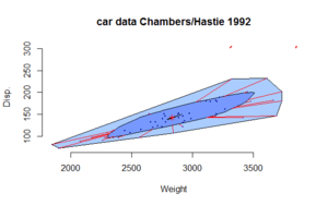
A bagplot, or starburst plot,[1][2] is a method in robust statistics for visualizing two- or three-dimensional statistical data, analogous to the one-dimensional box plot. Introduced in 1999 by Rousseuw et al., the bagplot allows one to visualize the location, spread, skewness, and outliers of a data set.[3]

Construction
The bagplot consists of three nested polygons, called the "bag", the "fence", and the "loop".
- The inner polygon, called the bag, is constructed on the basis of Tukey depth, the smallest number of observations that can be contained by a half-plane that also contains a given point.[4] It contains at most 50% of the data points
- The outermost of the three polygons, called the fence is not drawn as part of the bagplot, but is used to construct it. It is formed by inflating the bag by a certain factor (usually 3). Observations outside the fence are flagged as outliers.[5]
- The observations that are not marked as outliers are surrounded by a loop, the convex hull of the observations within the fence.[6]
An asterisk symbol (*) near the center of the graph is used to mark the depth median, the point with the highest possible Tukey depth. The observations between the bag and fence are marked by line segments, on a line to the depth median, connecting them to the bag.
The three-dimensional version consists of an inner and outer bag.[7] The outer bag must be drawn in transparent colors so that the inner bag remains visible.
Properties
The bagplot is invariant under affine transformations of the plane, and robust against outliers.[8]
References
- Rousseeuw, Peter J.; Ruts I.; Tukey J. W. (1999). "The Bagplot: A Bivariate Boxplot". The American Statistician. 53 (4): 382–387. doi:10.1080/00031305.1999.10474494.
- Ronald K. Pearson (1 April 2005). Mining Imperfect Data: Dealing with Contamination and Incomplete Records. SIAM. pp. 204–. ISBN 978-0-89871-582-8.
- Dominique Haughton; Jonathan Haughton (18 September 2011). Living Standards Analytics: Development through the Lens of Household Survey Data. Springer. pp. 14–. ISBN 978-1-4614-0385-2.
- Sophie Dabo-Niang; Frédéric Ferraty (21 May 2008). Functional and Operatorial Statistics. Springer. pp. 204–. ISBN 978-3-7908-2062-1.
- John C. Gower; Sugnet Gardner Lubbe; Niel J. Le Roux (23 February 2011). Understanding Biplots. John Wiley & Sons. pp. 59–. ISBN 978-1-119-97290-7.
- Prabhanjan Narayanachar Tattar (24 July 2013). R Statistical Application Development by Example Beginner's Guide. Packt Publishing Ltd. pp. 203–. ISBN 978-1-84951-945-8.
- Kruppa, Jochen J.; Jung K. (2017). "Automated multigroup outlier identification in molecular high-throughput data using bagplots and gemplots". BMC Bioinformatics. 18: 232. doi:10.1186/s12859-017-1645-5. PMC 5414140.
- Rajeev Raman; Robert Sedgewick; Matthias F. Stallmann (1 January 2006). Proceedings of the Eighth Workshop on Algorithm Engineering and Experiments and the Third Workshop on Analytic Algorithmics and Combinatorics. SIAM. pp. 62–. ISBN 978-0-89871-610-8.