Viscoelasticity

Viscoelasticity is the property of materials that exhibit both viscous and elastic characteristics when undergoing deformation. Viscous materials, like water, resist shear flow and strain linearly with time when a stress is applied. Elastic materials strain when stretched and immediately return to their original state once the stress is removed.

Viscoelastic materials have elements of both of these properties and, as such, exhibit time-dependent strain. Whereas elasticity is usually the result of bond stretching along crystallographic planes in an ordered solid, viscosity is the result of the diffusion of atoms or molecules inside an amorphous material.[1]

Background

In the nineteenth century, physicists such as Maxwell, Boltzmann, and Kelvin researched and experimented with creep and recovery of glasses, metals, and rubbers. Viscoelasticity was further examined in the late twentieth century when synthetic polymers were engineered and used in a variety of applications.[2] Viscoelasticity calculations depend heavily on the viscosity variable, η. The inverse of η is also known as fluidity, φ. The value of either can be derived as a function of temperature or as a given value (i.e. for a dashpot).[1]

Different types of responses (${\displaystyle \sigma }$) to a change in strain rate (d${\displaystyle \varepsilon }$/dt)

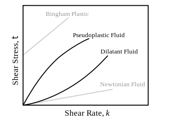
Depending on the change of strain rate versus stress inside a material the viscosity can be categorized as having a linear, non-linear, or plastic response. When a material exhibits a linear response it is categorized as a Newtonian material. In this case the stress is linearly proportional to the strain rate. If the material exhibits a non-linear response to the strain rate, it is categorized as Non-Newtonian fluid. There is also an interesting case where the viscosity decreases as the shear/strain rate remains constant. A material which exhibits this type of behavior is known as thixotropic. In addition, when the stress is independent of this strain rate, the material exhibits plastic deformation.[1] Many viscoelastic materials exhibit rubber like behavior explained by the thermodynamic theory of polymer elasticity.

Some examples of viscoelastic materials include amorphous polymers, semicrystalline polymers, biopolymers, metals at very high temperatures, and bitumen materials. Cracking occurs when the strain is applied quickly and outside of the elastic limit. Ligaments and tendons are viscoelastic, so the extent of the potential damage to them depends both on the rate of the change of their length as well as on the force applied.

A viscoelastic material has the following properties:

• hysteresis is seen in the stress–strain curve
• stress relaxation occurs: step constant strain causes decreasing stress
• creep occurs: step constant stress causes increasing strain

Elastic versus viscoelastic behavior

Stress–strain curves for a purely elastic material (a) and a viscoelastic material (b). The red area is a hysteresis loop and shows the amount of energy lost (as heat) in a loading and unloading cycle. It is equal to ${\displaystyle \oint \sigma \,d\varepsilon }$, where ${\displaystyle \sigma }$ is stress and ${\displaystyle \varepsilon }$ is strain.[1]

Unlike purely elastic substances, a viscoelastic substance has an elastic component and a viscous component. The viscosity of a viscoelastic substance gives the substance a strain rate dependence on time. Purely elastic materials do not dissipate energy (heat) when a load is applied, then removed. However, a viscoelastic substance dissipates energy when a load is applied, then removed. Hysteresis is observed in the stress–strain curve, with the area of the loop being equal to the energy lost during the loading cycle. Since viscosity is the resistance to thermally activated plastic deformation, a viscous material will lose energy through a loading cycle. Plastic deformation results in lost energy, which is uncharacteristic of a purely elastic material's reaction to a loading cycle.[1]

Specifically, viscoelasticity is a molecular rearrangement. When a stress is applied to a viscoelastic material such as a polymer, parts of the long polymer chain change positions. This movement or rearrangement is called creep. Polymers remain a solid material even when these parts of their chains are rearranging in order to accompany the stress, and as this occurs, it creates a back stress in the material. When the back stress is the same magnitude as the applied stress, the material no longer creeps. When the original stress is taken away, the accumulated back stresses will cause the polymer to return to its original form. The material creeps, which gives the prefix visco-, and the material fully recovers, which gives the suffix -elasticity.[2]

Types

Linear viscoelasticity is when the function is separable in both creep response and load. All linear viscoelastic models can be represented by a Volterra equation connecting stress and strain:

${\displaystyle \varepsilon (t)={\frac {\sigma (t)}{E_{\text{inst,creep}}}}+\int _{0}^{t}K(t-t^{\prime }){\dot {\sigma }}(t^{\prime })dt^{\prime }}$

or

${\displaystyle \sigma (t)=E_{\text{inst,relax}}\varepsilon (t)+\int _{0}^{t}F(t-t^{\prime }){\dot {\varepsilon }}(t^{\prime })dt^{\prime }}$

where

• t is time
• ${\displaystyle \sigma (t)}$ is stress
• ${\displaystyle \varepsilon (t)}$ is strain
• ${\displaystyle E_{\text{inst,creep}}}$ and ${\displaystyle E_{\text{inst,relax}}}$ are instantaneous elastic moduli for creep and relaxation
• K(t) is the creep function
• F(t) is the relaxation function

Linear viscoelasticity is usually applicable only for small deformations.

Nonlinear viscoelasticity is when the function is not separable. It usually happens when the deformations are large or if the material changes its properties under deformations.

An anelastic material is a special case of a viscoelastic material: an anelastic material will fully recover to its original state on the removal of load.

Dynamic modulus

Main article: Dynamic modulus

Viscoelasticity is studied using dynamic mechanical analysis, applying a small oscillatory stress and measuring the resulting strain.

• Purely elastic materials have stress and strain in phase, so that the response of one caused by the other is immediate.
• In purely viscous materials, strain lags stress by a 90 degree phase.
• Viscoelastic materials exhibit behavior somewhere in the middle of these two types of material, exhibiting some lag in strain.

A complex dynamic modulus G can be used to represent the relations between the oscillating stress and strain:

${\displaystyle G=G'+iG''}$

where ${\displaystyle i^{2}=-1}$; ${\displaystyle G'}$ is the storage modulus and ${\displaystyle G''}$ is the loss modulus:

${\displaystyle G'={\frac {\sigma _{0}}{\varepsilon _{0}}}\cos \delta }$

${\displaystyle G''={\frac {\sigma _{0}}{\varepsilon _{0}}}\sin \delta }$

where ${\displaystyle \sigma _{0}}$ and ${\displaystyle \varepsilon _{0}}$ are the amplitudes of stress and strain respectively, and ${\displaystyle \delta }$ is the phase shift between them.

Constitutive models of linear viscoelasticity

Comparison of creep and stress relaxation for three and four element models

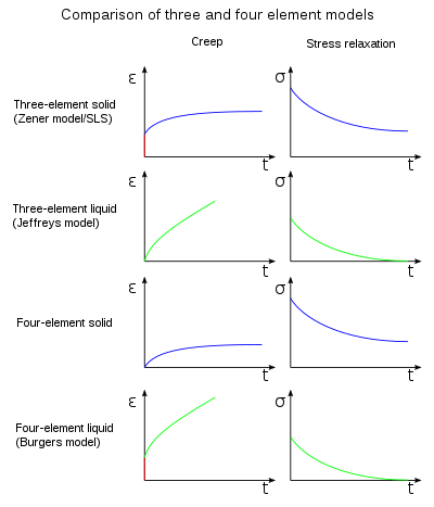
Viscoelastic materials, such as amorphous polymers, semicrystalline polymers, biopolymers and even the living tissue and cells,[3] can be modeled in order to determine their stress and strain or force and displacement interactions as well as their temporal dependencies. These models, which include the Maxwell model, the Kelvin–Voigt model, the standard linear solid model, and the Burgers model, are used to predict a material's response under different loading conditions. Viscoelastic behavior has elastic and viscous components modeled as linear combinations of springs and dashpots, respectively. Each model differs in the arrangement of these elements, and all of these viscoelastic models can be equivalently modeled as electrical circuits. In an equivalent electrical circuit, stress is represented by voltage, and strain rate by current. The elastic modulus of a spring is analogous to a circuit's capacitance (it stores energy) and the viscosity of a dashpot to a circuit's resistance (it dissipates energy).

The elastic components, as previously mentioned, can be modeled as springs of elastic constant E, given the formula:

${\displaystyle \sigma =E\varepsilon }$

where σ is the stress, E is the elastic modulus of the material, and ε is the strain that occurs under the given stress, similar to Hooke's law.

The viscous components can be modeled as dashpots such that the stress–strain rate relationship can be given as,

${\displaystyle \sigma =\eta {\frac {d\varepsilon }{dt}}}$

where σ is the stress, η is the viscosity of the material, and dε/dt is the time derivative of strain.

The relationship between stress and strain can be simplified for specific stress rates. For high stress states/short time periods, the time derivative components of the stress–strain relationship dominate. A dashpot resists changes in length, and in a high stress state it can be approximated as a rigid rod. Since a rigid rod cannot be stretched past its original length, no strain is added to the system.[4]

Conversely, for low stress states/longer time periods, the time derivative components are negligible and the dashpot can be effectively removed from the system - an "open" circuit. As a result, only the spring connected in parallel to the dashpot will contribute to the total strain in the system.[4]

Maxwell model

Main article: Maxwell material

Maxwell model

The Maxwell model can be represented by a purely viscous damper and a purely elastic spring connected in series, as shown in the diagram. The model can be represented by the following equation:

${\displaystyle \sigma +{\frac {\eta }{E}}{\dot {\sigma }}=\eta {\dot {\varepsilon }}}$

Under this model, if the material is put under a constant strain, the stresses gradually relax. When a material is put under a constant stress, the strain has two components. First, an elastic component occurs instantaneously, corresponding to the spring, and relaxes immediately upon release of the stress. The second is a viscous component that grows with time as long as the stress is applied. The Maxwell model predicts that stress decays exponentially with time, which is accurate for most polymers. One limitation of this model is that it does not predict creep accurately. The Maxwell model for creep or constant-stress conditions postulates that strain will increase linearly with time. However, polymers for the most part show the strain rate to be decreasing with time.[2]

Applications to soft solids: thermoplastic polymers in the vicinity of their melting temperature, fresh concrete (neglecting its aging), numerous metals at a temperature close to their melting point.

Kelvin–Voigt model

Main article: Kelvin–Voigt material

Schematic representation of Kelvin–Voigt model.

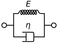
The Kelvin–Voigt model, also known as the Voigt model, consists of a Newtonian damper and Hookean elastic spring connected in parallel, as shown in the picture. It is used to explain the creep behaviour of polymers.

The constitutive relation is expressed as a linear first-order differential equation:

${\displaystyle \sigma =E\varepsilon +\eta {\dot {\varepsilon }}}$

This model represents a solid undergoing reversible, viscoelastic strain. Upon application of a constant stress, the material deforms at a decreasing rate, asymptotically approaching the steady-state strain. When the stress is released, the material gradually relaxes to its undeformed state. At constant stress (creep), the model is quite realistic as it predicts strain to tend to σ/E as time continues to infinity. Similar to the Maxwell model, the Kelvin–Voigt model also has limitations. The model is extremely good with modelling creep in materials, but with regards to relaxation the model is much less accurate.[5]

Applications: organic polymers, rubber, wood when the load is not too high.

Standard linear solid model

Main article: Standard linear solid model

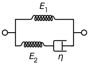
The standard linear solid model, also known as the Zener model, consists of two springs and a dashpot. It is the simplest model that describes both the creep and stress relaxation behaviors of a viscoelastic material properly. For this model, the governing constitutive relations are:

Maxwell representation	Kelvin representation
${\displaystyle \sigma +{\frac {\eta }{E_{2}}}{\dot {\sigma }}=E_{1}\varepsilon +{\frac {\eta (E_{1}+E_{2})}{E_{2}}}{\dot {\varepsilon }}}$	${\displaystyle \sigma +{\frac {\eta }{E_{1}+E_{2}}}{\dot {\sigma }}={\frac {E_{1}E_{2}}{E_{1}+E_{2}}}\varepsilon +{\frac {E_{1}\eta }{E_{1}+E_{2}}}{\dot {\varepsilon }}}$

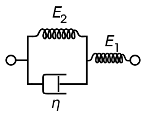Under a constant stress, the modeled material will instantaneously deform to some strain, which is the instantaneous elastic portion of the strain. After that it will continue to deform and asymptotically approach a steady-state strain, which is the retarded elastic portion of the strain. Although the Standard Linear Solid Model is more accurate than the Maxwell and Kelvin–Voigt models in predicting material responses, mathematically it returns inaccurate results for strain under specific loading conditions.

Burgers model

Main article: Burgers material

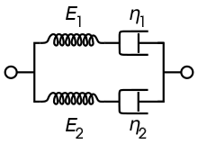
The Burgers model consists of either two Maxwell components in parallel or a Kelvin–Voigt component, a spring and a dashpot in series. For this model, the governing constitutive relations are:

Maxwell representation	Kelvin representation
${\displaystyle \sigma +\left({\frac {\eta _{1}}{E_{1}}}+{\frac {\eta _{2}}{E_{2}}}\right){\dot {\sigma }}+{\frac {\eta _{1}\eta _{2}}{E_{1}E_{2}}}{\ddot {\sigma }}=\left(\eta _{1}+\eta _{2}\right){\dot {\varepsilon }}+{\frac {\eta _{1}\eta _{2}\left(E_{1}+E_{2}\right)}{E_{1}E_{2}}}{\ddot {\varepsilon }}}$	${\displaystyle \sigma +\left({\frac {\eta _{1}}{E_{1}}}+{\frac {\eta _{2}}{E_{1}}}+{\frac {\eta _{2}}{E_{2}}}\right){\dot {\sigma }}+{\frac {\eta _{1}\eta _{2}}{E_{1}E_{2}}}{\ddot {\sigma }}=\eta _{2}{\dot {\varepsilon }}+{\frac {\eta _{1}\eta _{2}}{E_{1}}}{\ddot {\varepsilon }}}$

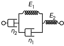This model incorporates viscous flow into the standard linear solid model, giving a linearly increasing asymptote for strain under fixed loading conditions.

Generalized Maxwell model

Main article: Generalized Maxwell model

Schematic of Maxwell-Wiechert Model

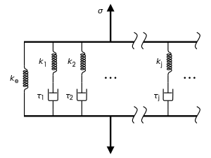
The Generalized Maxwell model, also known as the Wiechert model, is the most general form of the linear model for viscoelasticity. It takes into account that the relaxation does not occur at a single time, but at a distribution of times. Due to molecular segments of different lengths with shorter ones contributing less than longer ones, there is a varying time distribution. The Wiechert model shows this by having as many spring–dashpot Maxwell elements as necessary to accurately represent the distribution. The figure on the right shows the generalised Wiechert model.[6] Applications: metals and alloys at temperatures lower than one quarter of their absolute melting temperature (expressed in K).

Prony series

Main article: Prony's method

In a one-dimensional relaxation test, the material is subjected to a sudden strain that is kept constant over the duration of the test, and the stress is measured over time. The initial stress is due to the elastic response of the material. Then, the stress relaxes over time due to the viscous effects in the material. Typically, either a tensile, compressive, bulk compression, or shear strain is applied. The resulting stress vs. time data can be fitted with a number of equations, called models. Only the notation changes depending of the type of strain applied: tensile-compressive relaxation is denoted ${\displaystyle E}$, shear is denoted ${\displaystyle G}$, bulk is denoted ${\displaystyle K}$. The Prony series for the shear relaxation is

${\displaystyle G(t)=G_{\infty }+\Sigma _{i=1}^{N}G_{i}\exp(-t/\tau _{i})}$

where ${\displaystyle G_{\infty }}$ is the long term modulus once the material is totally relaxed, ${\displaystyle \tau _{i}}$ are the relaxation times (not to be confused with ${\displaystyle \tau _{i}}$ in the diagram); the higher their values, the longer it takes for the stress to relax. The data is fitted with the equation by using a minimization algorithm that adjust the parameters (${\displaystyle G_{\infty },G_{i},\tau _{i}}$) to minimize the error between the predicted and data values.[7]

An alternative form is obtained noting that the elastic modulus is related to the long term modulus by

${\displaystyle G(t=0)=G_{0}=G_{\infty }+\Sigma _{i=1}^{N}G_{i}}$

Therefore,

${\displaystyle G(t)=G_{0}-\Sigma _{i=1}^{N}G_{i}[1-\exp(-t/\tau _{i})]}$

This form is convenient when the elastic shear modulus ${\displaystyle G_{0}}$ is obtained from data independent from the relaxation data, and/or for computer implementation, when it is desired to specify the elastic properties separately from the viscous properties, as in.[8]

A creep experiment is usually easier to perform than a relaxation one, so most data is available as (creep) compliance vs. time.[9] Unfortunately, there is no known closed form for the (creep) compliance in terms of the coefficient of the Prony series. So, if one has creep data, it is not easy to get the coefficients of the (relaxation) Prony series, which are needed for example in.[8] An expedient way to obtain these coefficients is the following. First, fit the creep data with a model that has closed form solutions in both compliance and relaxation; for example the Maxwell-Kelvin model (eq. 7.18-7.19) in[10] or the Standard Solid Model (eq. 7.20-7.21) in[10] (section 7.1.3). Once the parameters of the creep model are known, produce relaxation pseudo-data with the conjugate relaxation model for the same times of the original data. Finally, fit the pseudo data with the Prony series.

Effect of temperature on viscoelastic behavior

Main article: Time–temperature superposition

The secondary bonds of a polymer constantly break and reform due to thermal motion. Application of a stress favors some conformations over others, so the molecules of the polymer will gradually "flow" into the favored conformations over time.[11] Because thermal motion is one factor contributing to the deformation of polymers, viscoelastic properties change with increasing or decreasing temperature. In most cases, the creep modulus, defined as the ratio of applied stress to the time-dependent strain, decreases with increasing temperature. Generally speaking, an increase in temperature correlates to a logarithmic decrease in the time required to impart equal strain under a constant stress. In other words, it takes less work to stretch a viscoelastic material an equal distance at a higher temperature than it does at a lower temperature.

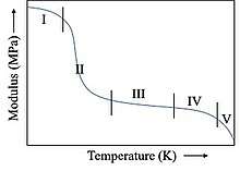
More detailed effect of temperature on the viscoelastic behavior of polymer can be plotted as shown.

There are mainly five regions (some denoted four, which combines VI and V together) included in the typical polymers[12].

Region I: Glassy state of the polymer is presented in this region. The temperature in this region for a given polymer is too low to endow molecular motion. Hence the motion of the molecules is frozen in this area. The mechanical property is hard and brittle in this region[13].

Region II: Polymer passes glass transition temperature in this region. Beyond Tg, the thermal energy provided by the environment is enough to unfreeze the motion of molecules. The molecules are allowed to have local motion in this region hence leading to a sharp drop in stiffness compared to Region I.

Region III: Rubbery plateau region. Materials lie in this region would exist long-range elasticity driven by entropy. For instance, a rubber band is disordered in the initial state of this region. When stretching the rubber band, you also align the structure to be more ordered. Therefore, when releasing the rubber band, it will spontaneously seek higher entropy state hence goes back to its initial state. This is what we called entropy-driven elasticity shape recovery.

Region IV: The behavior in the rubbery flow region is highly time-dependent. Polymers in this region would need to use a time-temperature superposition to get more detailed information to cautiously decide how to use the materials. For instance, if the material is used to cope with short interaction time purpose, it could present as 'hard' material. While using for long interaction time purposes, it would act as 'soft' material[14].

Region V: Viscous polymer flows easily in this region. Another significant drop in stiffness.

Temperature dependence of modulus

Extreme cold temperatures can cause viscoelastic materials to change to the glass phase and become brittle. For example, exposure of pressure sensitive adhesives to extreme cold (dry ice, freeze spray, etc.) causes them to lose their tack, resulting in debonding.

Viscoelastic creep

Main article: Creep (deformation)

a) Applied stress and b) induced strain (b) as functions of time over a short period for a viscoelastic material.

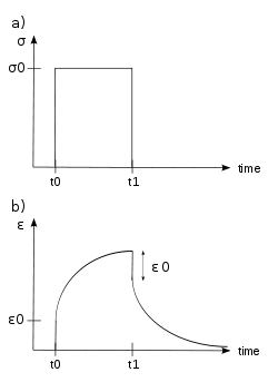
When subjected to a step constant stress, viscoelastic materials experience a time-dependent increase in strain. This phenomenon is known as viscoelastic creep.

At time ${\displaystyle t_{0}}$, a viscoelastic material is loaded with a constant stress that is maintained for a sufficiently long time period. The material responds to the stress with a strain that increases until the material ultimately fails, if it is a viscoelastic liquid. If, on the other hand, it is a viscoelastic solid, it may or may not fail depending on the applied stress versus the material's ultimate resistance. When the stress is maintained for a shorter time period, the material undergoes an initial strain until a time ${\displaystyle t_{1}}$, after which the strain immediately decreases (discontinuity) then gradually decreases at times ${\displaystyle t>t_{1}}$ to a residual strain.

Viscoelastic creep data can be presented by plotting the creep modulus (constant applied stress divided by total strain at a particular time) as a function of time.[15] Below its critical stress, the viscoelastic creep modulus is independent of stress applied. A family of curves describing strain versus time response to various applied stress may be represented by a single viscoelastic creep modulus versus time curve if the applied stresses are below the material's critical stress value.

Viscoelastic creep is important when considering long-term structural design. Given loading and temperature conditions, designers can choose materials that best suit component lifetimes.

Measurement

Though there are many instruments that test the mechanical and viscoelastic response of materials, broadband viscoelastic spectroscopy (BVS) and resonant ultrasound spectroscopy (RUS) are more commonly used to test viscoelastic behavior because they can be used above and below ambient temperatures and are more specific to testing viscoelasticity. These two instruments employ a damping mechanism at various frequencies and time ranges with no appeal to time–temperature superposition. Using BVS and RUS to study the mechanical properties of materials is important to understanding how a material exhibiting viscoelasticity will perform.[16]

See also

• Bingham plastic
• Biomaterial
• Biomechanics
• Blood viscoelasticity
• Constant viscosity elastic fluids
• Glass transition
• Pressure-sensitive adhesive
• Rheology
• Rubber elasticity
• Silly Putty
• Viscoelasticity of bone
• Viscoplasticity

References

1. Meyers and Chawla (1999): "Mechanical Behavior of Materials", 98-103.
2. McCrum, Buckley, and Bucknell (2003): "Principles of Polymer Engineering," 117-176.
3. Biswas, Abhijit; Manivannan, M.; Srinivasan, Mandyam A. (2015). "Multiscale Layered Biomechanical Model of the Pacinian Corpuscle". IEEE Transactions on Haptics. 8 (1): 31–42. doi:10.1109/TOH.2014.2369416. PMID 25398182.
4. Van Vliet, Krystyn J. (2006); "3.032 Mechanical Behavior of Materials"
5. Tanner, Roger I. (1988). Engineering Rheologu. Oxford University Press. p. 27. ISBN 0-19-856197-0.
6. Roylance, David (2001); "Engineering Viscoelasticity", 14-15
7. E. J. Barbero. Time-temperature-age Superposition Principle for Predicting Long-term Response of Linear Viscoelastic Materials, chapter 2 in Creep and fatigue in polymer matrix composites. Woodhead, 2011..
8. Simulia. Abaqus Analysis User's Manual, 19.7.1 Time domain vicoelasticity, 6.10 edition, 2010
9. Computer Aided Material Preselection by Uniform Standards
10. E. J. Barbero. Finite Element Analysis of Composite Materials. CRC Press, Boca Raton, Florida, 2007.
11. S.A. Baeurle, A. Hotta, A.A. Gusev, Polymer 47, 6243-6253 (2006).
12. Aklonis., J.J. (1981). "Mechanical properties of polymer". J Chem Educ. 58:892.
13. I. M., Kalogeras (2012). "The nature of the glassy state: structure and glass transitions". Journal of Materials Education. 34(3), 69.
14. I, Emri (2010). Time-dependent behavior of solid polymers.
15. Rosato, et al. (2001): "Plastics Design Handbook", 63-64.
16. Rod Lakes (1998). Viscoelastic solids. CRC Press. ISBN 0-8493-9658-1.

• Silbey and Alberty (2001): Physical Chemistry, 857. John Wiley & Sons, Inc.
• Alan S. Wineman and K. R. Rajagopal (2000): Mechanical Response of Polymers: An Introduction
• Allen and Thomas (1999): The Structure of Materials, 51.
• Crandal et al. (1999): An Introduction to the Mechanics of Solids 348
• J. Lemaitre and J. L. Chaboche (1994) Mechanics of solid materials
• Yu. Dimitrienko (2011) Nonlinear continuum mechanics and Large Inelastic Deformations, Springer, 772p