Mixture model

In statistics, a mixture model is a probabilistic model for representing the presence of subpopulations within an overall population, without requiring that an observed data set should identify the sub-population to which an individual observation belongs. Formally a mixture model corresponds to the mixture distribution that represents the probability distribution of observations in the overall population. However, while problems associated with "mixture distributions" relate to deriving the properties of the overall population from those of the sub-populations, "mixture models" are used to make statistical inferences about the properties of the sub-populations given only observations on the pooled population, without sub-population identity information.

Not to be confused with mixed model.

See also: Mixture distribution

Some ways of implementing mixture models involve steps that attribute postulated sub-population-identities to individual observations (or weights towards such sub-populations), in which case these can be regarded as types of unsupervised learning or clustering procedures. However, not all inference procedures involve such steps.

Mixture models should not be confused with models for compositional data, i.e., data whose components are constrained to sum to a constant value (1, 100%, etc.). However, compositional models can be thought of as mixture models, where members of the population are sampled at random. Conversely, mixture models can be thought of as compositional models, where the total size reading population has been normalized to 1.

Structure

General mixture model

A typical finite-dimensional mixture model is a hierarchical model consisting of the following components:

• N random variables that are observed, each distributed according to a mixture of K components, with the components belonging to the same parametric family of distributions (e.g., all normal, all Zipfian, etc.) but with different parameters
• N random latent variables specifying the identity of the mixture component of each observation, each distributed according to a K-dimensional categorical distribution
• A set of K mixture weights, which are probabilities that sum to 1.
• A set of K parameters, each specifying the parameter of the corresponding mixture component. In many cases, each "parameter" is actually a set of parameters. For example, if the mixture components are Gaussian distributions, there will be a mean and variance for each component. If the mixture components are categorical distributions (e.g., when each observation is a token from a finite alphabet of size V), there will be a vector of V probabilities summing to 1.

In addition, in a Bayesian setting, the mixture weights and parameters will themselves be random variables, and prior distributions will be placed over the variables. In such a case, the weights are typically viewed as a K-dimensional random vector drawn from a Dirichlet distribution (the conjugate prior of the categorical distribution), and the parameters will be distributed according to their respective conjugate priors.

Mathematically, a basic parametric mixture model can be described as follows:

${\displaystyle {\begin{array}{lcl}K&=&{\text{number of mixture components}}\\N&=&{\text{number of observations}}\\\theta _{i=1\dots K}&=&{\text{parameter of distribution of observation associated with component }}i\\\phi _{i=1\dots K}&=&{\text{mixture weight, i.e., prior probability of a particular component }}i\\{\boldsymbol {\phi }}&=&K{\text{-dimensional vector composed of all the individual }}\phi _{1\dots K}{\text{; must sum to 1}}\\z_{i=1\dots N}&=&{\text{component of observation }}i\\x_{i=1\dots N}&=&{\text{observation }}i\\F(x|\theta )&=&{\text{probability distribution of an observation, parametrized on }}\theta \\z_{i=1\dots N}&\sim &\operatorname {Categorical} ({\boldsymbol {\phi }})\\x_{i=1\dots N}|z_{i=1\dots N}&\sim &F(\theta _{z_{i}})\end{array}}}$

In a Bayesian setting, all parameters are associated with random variables, as follows:

${\displaystyle {\begin{array}{lcl}K,N&=&{\text{as above}}\\\theta _{i=1\dots K},\phi _{i=1\dots K},{\boldsymbol {\phi }}&=&{\text{as above}}\\z_{i=1\dots N},x_{i=1\dots N},F(x|\theta )&=&{\text{as above}}\\\alpha &=&{\text{shared hyperparameter for component parameters}}\\\beta &=&{\text{shared hyperparameter for mixture weights}}\\H(\theta |\alpha )&=&{\text{prior probability distribution of component parameters, parametrized on }}\alpha \\\theta _{i=1\dots K}&\sim &H(\theta |\alpha )\\{\boldsymbol {\phi }}&\sim &\operatorname {Symmetric-Dirichlet} _{K}(\beta )\\z_{i=1\dots N}|{\boldsymbol {\phi }}&\sim &\operatorname {Categorical} ({\boldsymbol {\phi }})\\x_{i=1\dots N}|z_{i=1\dots N},\theta _{i=1\dots K}&\sim &F(\theta _{z_{i}})\end{array}}}$

This characterization uses F and H to describe arbitrary distributions over observations and parameters, respectively. Typically H will be the conjugate prior of F. The two most common choices of F are Gaussian aka "normal" (for real-valued observations) and categorical (for discrete observations). Other common possibilities for the distribution of the mixture components are:

• Binomial distribution, for the number of "positive occurrences" (e.g., successes, yes votes, etc.) given a fixed number of total occurrences
• Multinomial distribution, similar to the binomial distribution, but for counts of multi-way occurrences (e.g., yes/no/maybe in a survey)
• Negative binomial distribution, for binomial-type observations but where the quantity of interest is the number of failures before a given number of successes occurs
• Poisson distribution, for the number of occurrences of an event in a given period of time, for an event that is characterized by a fixed rate of occurrence
• Exponential distribution, for the time before the next event occurs, for an event that is characterized by a fixed rate of occurrence
• Log-normal distribution, for positive real numbers that are assumed to grow exponentially, such as incomes or prices
• Multivariate normal distribution (aka multivariate Gaussian distribution), for vectors of correlated outcomes that are individually Gaussian-distributed
• Multivariate Student's-t distribution (aka multivariate t-distribution), for vectors of heavy-tailed correlated outcomes[1]
• A vector of Bernoulli-distributed values, corresponding, e.g., to a black-and-white image, with each value representing a pixel; see the handwriting-recognition example below

Specific examples

Gaussian mixture model

Non-Bayesian Gaussian mixture model using plate notation. Smaller squares indicate fixed parameters; larger circles indicate random variables. Filled-in shapes indicate known values. The indication [K] means a vector of size K.

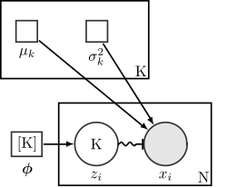
A typical non-Bayesian Gaussian mixture model looks like this:

${\displaystyle {\begin{array}{lcl}K,N&=&{\text{as above}}\\\phi _{i=1\dots K},{\boldsymbol {\phi }}&=&{\text{as above}}\\z_{i=1\dots N},x_{i=1\dots N}&=&{\text{as above}}\\\theta _{i=1\dots K}&=&\{\mu _{i=1\dots K},\sigma _{i=1\dots K}^{2}\}\\\mu _{i=1\dots K}&=&{\text{mean of component }}i\\\sigma _{i=1\dots K}^{2}&=&{\text{variance of component }}i\\z_{i=1\dots N}&\sim &\operatorname {Categorical} ({\boldsymbol {\phi }})\\x_{i=1\dots N}&\sim &{\mathcal {N}}(\mu _{z_{i}},\sigma _{z_{i}}^{2})\end{array}}}$

Bayesian Gaussian mixture model using plate notation. Smaller squares indicate fixed parameters; larger circles indicate random variables. Filled-in shapes indicate known values. The indication [K] means a vector of size K.

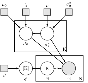
A Bayesian version of a Gaussian mixture model is as follows:

${\displaystyle {\begin{array}{lcl}K,N&=&{\text{as above}}\\\phi _{i=1\dots K},{\boldsymbol {\phi }}&=&{\text{as above}}\\z_{i=1\dots N},x_{i=1\dots N}&=&{\text{as above}}\\\theta _{i=1\dots K}&=&\{\mu _{i=1\dots K},\sigma _{i=1\dots K}^{2}\}\\\mu _{i=1\dots K}&=&{\text{mean of component }}i\\\sigma _{i=1\dots K}^{2}&=&{\text{variance of component }}i\\\mu _{0},\lambda ,\nu ,\sigma _{0}^{2}&=&{\text{shared hyperparameters}}\\\mu _{i=1\dots K}&\sim &{\mathcal {N}}(\mu _{0},\lambda \sigma _{i}^{2})\\\sigma _{i=1\dots K}^{2}&\sim &\operatorname {Inverse-Gamma} (\nu ,\sigma _{0}^{2})\\{\boldsymbol {\phi }}&\sim &\operatorname {Symmetric-Dirichlet} _{K}(\beta )\\z_{i=1\dots N}&\sim &\operatorname {Categorical} ({\boldsymbol {\phi }})\\x_{i=1\dots N}&\sim &{\mathcal {N}}(\mu _{z_{i}},\sigma _{z_{i}}^{2})\end{array}}}$

Multivariate Gaussian mixture model

A Bayesian Gaussian mixture model is commonly extended to fit a vector of unknown parameters (denoted in bold), or multivariate normal distributions. In a multivariate distribution (i.e. one modelling a vector ${\displaystyle {\boldsymbol {x}}}$ with N random variables) one may model a vector of parameters (such as several observations of a signal or patches within an image) using a Gaussian mixture model prior distribution on the vector of estimates given by

${\displaystyle p({\boldsymbol {\theta }})=\sum _{i=1}^{K}\phi _{i}{\mathcal {N}}({\boldsymbol {\mu _{i},\Sigma _{i}}})}$

where the i^th vector component is characterized by normal distributions with weights ${\displaystyle \phi _{i}}$, means ${\displaystyle {\boldsymbol {\mu _{i}}}}$ and covariance matrices ${\displaystyle {\boldsymbol {\Sigma _{i}}}}$. To incorporate this prior into a Bayesian estimation, the prior is multiplied with the known distribution ${\displaystyle p({\boldsymbol {x|\theta }})}$ of the data ${\displaystyle {\boldsymbol {x}}}$ conditioned on the parameters ${\displaystyle {\boldsymbol {\theta }}}$ to be estimated. With this formulation, the posterior distribution ${\displaystyle p({\boldsymbol {\theta |x}})}$ is also a Gaussian mixture model of the form

${\displaystyle p({\boldsymbol {\theta |x}})=\sum _{i=1}^{K}{\tilde {\phi _{i}}}{\mathcal {N}}({\boldsymbol {{\tilde {\mu _{i}}},{\tilde {\Sigma _{i}}}}})}$

with new parameters ${\displaystyle {\tilde {\phi _{i}}},{\boldsymbol {\tilde {\mu _{i}}}}}$ and ${\displaystyle {\boldsymbol {\tilde {\Sigma _{i}}}}}$ that are updated using the EM algorithm. [2] Although EM-based parameter updates are well-established, providing the initial estimates for these parameters is currently an area of active research. Note that this formulation yields a closed-form solution to the complete posterior distribution. Estimations of the random variable ${\displaystyle {\boldsymbol {\theta }}}$ may be obtained via one of several estimators, such as the mean or maximum of the posterior distribution.

Such distributions are useful for assuming patch-wise shapes of images and clusters, for example. In the case of image representation, each Gaussian may be tilted, expanded, and warped according to the covariance matrices ${\displaystyle {\boldsymbol {\Sigma _{i}}}}$. One Gaussian distribution of the set is fit to each patch (usually of size 8x8 pixels) in the image. Notably, any distribution of points around a cluster (see k-means) may be accurately given enough Gaussian components, but scarcely over K=20 components are needed to accurately model a given image distribution or cluster of data.

Categorical mixture model

Non-Bayesian categorical mixture model using plate notation. Smaller squares indicate fixed parameters; larger circles indicate random variables. Filled-in shapes indicate known values. The indication [K] means a vector of size K; likewise for [V].

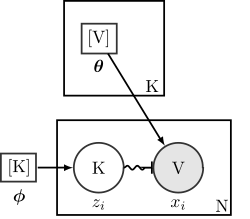
A typical non-Bayesian mixture model with categorical observations looks like this:

• ${\displaystyle K,N:}$ as above
• ${\displaystyle \phi _{i=1\dots K},{\boldsymbol {\phi }}:}$ as above
• ${\displaystyle z_{i=1\dots N},x_{i=1\dots N}:}$ as above
• ${\displaystyle V:}$ dimension of categorical observations, e.g., size of word vocabulary
• ${\displaystyle \theta _{i=1\dots K,j=1\dots V}:}$ probability for component ${\displaystyle i}$ of observing item ${\displaystyle j}$
• ${\displaystyle {\boldsymbol {\theta }}_{i=1\dots K}:}$ vector of dimension ${\displaystyle V,}$ composed of ${\displaystyle \theta _{i,1\dots V};}$ must sum to 1

The random variables:

${\displaystyle {\begin{array}{lcl}z_{i=1\dots N}&\sim &\operatorname {Categorical} ({\boldsymbol {\phi }})\\x_{i=1\dots N}&\sim &{\text{Categorical}}({\boldsymbol {\theta }}_{z_{i}})\end{array}}}$

Bayesian categorical mixture model using plate notation. Smaller squares indicate fixed parameters; larger circles indicate random variables. Filled-in shapes indicate known values. The indication [K] means a vector of size K; likewise for [V].

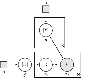
A typical Bayesian mixture model with categorical observations looks like this:

• ${\displaystyle K,N:}$ as above
• ${\displaystyle \phi _{i=1\dots K},{\boldsymbol {\phi }}:}$ as above
• ${\displaystyle z_{i=1\dots N},x_{i=1\dots N}:}$ as above
• ${\displaystyle V:}$ dimension of categorical observations, e.g., size of word vocabulary
• ${\displaystyle \theta _{i=1\dots K,j=1\dots V}:}$ probability for component ${\displaystyle i}$ of observing item ${\displaystyle j}$
• ${\displaystyle {\boldsymbol {\theta }}_{i=1\dots K}:}$ vector of dimension ${\displaystyle V,}$ composed of ${\displaystyle \theta _{i,1\dots V};}$ must sum to 1
• ${\displaystyle \alpha$ :} shared concentration hyperparameter of ${\displaystyle {\boldsymbol {\theta }}}$ for each component
• ${\displaystyle \beta$ :} concentration hyperparameter of ${\displaystyle {\boldsymbol {\phi }}}$

The random variables:

${\displaystyle {\begin{array}{lcl}{\boldsymbol {\phi }}&\sim &\operatorname {Symmetric-Dirichlet} _{K}(\beta )\\{\boldsymbol {\theta }}_{i=1\dots K}&\sim &{\text{Symmetric-Dirichlet}}_{V}(\alpha )\\z_{i=1\dots N}&\sim &\operatorname {Categorical} ({\boldsymbol {\phi }})\\x_{i=1\dots N}&\sim &{\text{Categorical}}({\boldsymbol {\theta }}_{z_{i}})\end{array}}}$

Examples

A financial model

The normal distribution is plotted using different means and variances

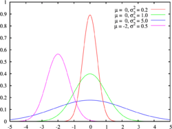
Financial returns often behave differently in normal situations and during crisis times. A mixture model[3] for return data seems reasonable. Sometimes the model used is a jump-diffusion model, or as a mixture of two normal distributions. See Financial economics#Challenges and criticism for further context.

House prices

Assume that we observe the prices of N different houses. Different types of houses in different neighborhoods will have vastly different prices, but the price of a particular type of house in a particular neighborhood (e.g., three-bedroom house in moderately upscale neighborhood) will tend to cluster fairly closely around the mean. One possible model of such prices would be to assume that the prices are accurately described by a mixture model with K different components, each distributed as a normal distribution with unknown mean and variance, with each component specifying a particular combination of house type/neighborhood. Fitting this model to observed prices, e.g., using the expectation-maximization algorithm, would tend to cluster the prices according to house type/neighborhood and reveal the spread of prices in each type/neighborhood. (Note that for values such as prices or incomes that are guaranteed to be positive and which tend to grow exponentially, a log-normal distribution might actually be a better model than a normal distribution.)

Topics in a document

Assume that a document is composed of N different words from a total vocabulary of size V, where each word corresponds to one of K possible topics. The distribution of such words could be modelled as a mixture of K different V-dimensional categorical distributions. A model of this sort is commonly termed a topic model. Note that expectation maximization applied to such a model will typically fail to produce realistic results, due (among other things) to the excessive number of parameters. Some sorts of additional assumptions are typically necessary to get good results. Typically two sorts of additional components are added to the model:

1. A prior distribution is placed over the parameters describing the topic distributions, using a Dirichlet distribution with a concentration parameter that is set significantly below 1, so as to encourage sparse distributions (where only a small number of words have significantly non-zero probabilities).
2. Some sort of additional constraint is placed over the topic identities of words, to take advantage of natural clustering.

• For example, a Markov chain could be placed on the topic identities (i.e., the latent variables specifying the mixture component of each observation), corresponding to the fact that nearby words belong to similar topics. (This results in a hidden Markov model, specifically one where a prior distribution is placed over state transitions that favors transitions that stay in the same state.)
• Another possibility is the latent Dirichlet allocation model, which divides up the words into D different documents and assumes that in each document only a small number of topics occur with any frequency.

Handwriting recognition

The following example is based on an example in Christopher M. Bishop, Pattern Recognition and Machine Learning.[4]

Imagine that we are given an N×N black-and-white image that is known to be a scan of a hand-written digit between 0 and 9, but we don't know which digit is written. We can create a mixture model with ${\displaystyle K=10}$ different components, where each component is a vector of size ${\displaystyle N^{2}}$ of Bernoulli distributions (one per pixel). Such a model can be trained with the expectation-maximization algorithm on an unlabeled set of hand-written digits, and will effectively cluster the images according to the digit being written. The same model could then be used to recognize the digit of another image simply by holding the parameters constant, computing the probability of the new image for each possible digit (a trivial calculation), and returning the digit that generated the highest probability.

Assessing projectile accuracy (a.k.a. circular error probable, CEP)

Mixture models apply in the problem of directing multiple projectiles at a target (as in air, land, or sea defense applications), where the physical and/or statistical characteristics of the projectiles differ within the multiple projectiles. An example might be shots from multiple munitions types or shots from multiple locations directed at one target. The combination of projectile types may be characterized as a Gaussian mixture model.[5] Further, a well-known measure of accuracy for a group of projectiles is the circular error probable (CEP), which is the number R such that, on average, half of the group of projectiles falls within the circle of radius R about the target point. The mixture model can be used to determine (or estimate) the value R. The mixture model properly captures the different types of projectiles.

Direct and indirect applications

The financial example above is one direct application of the mixture model, a situation in which we assume an underlying mechanism so that each observation belongs to one of some number of different sources or categories. This underlying mechanism may or may not, however, be observable. In this form of mixture, each of the sources is described by a component probability density function, and its mixture weight is the probability that an observation comes from this component.

In an indirect application of the mixture model we do not assume such a mechanism. The mixture model is simply used for its mathematical flexibilities. For example, a mixture of two normal distributions with different means may result in a density with two modes, which is not modeled by standard parametric distributions. Another example is given by the possibility of mixture distributions to model fatter tails than the basic Gaussian ones, so as to be a candidate for modeling more extreme events. When combined with dynamical consistency, this approach has been applied to financial derivatives valuation in presence of the volatility smile in the context of local volatility models. This defines our application.

Predictive Maintenance

The mixture model-based clustering is also predominantly used in identifying the state of the machine in predictive maintenance. Density plots are used to analyze the density of high dimensional features. If multi-model densities are observed, then it is assumed that a finite set of densities are formed by a finite set of normal mixtures. A multivariate Gaussian mixture model is used to cluster the feature data into k number of groups where k represents each state of the machine. The machine state can be a normal state, power off state, or faulty state.[6] Each formed cluster can be diagnosed using techniques such as spectral analysis. In the recent years, this has also been widely used in other areas such as early fault detection.[7]

Fuzzy image segmentation

An example of Gaussian Mixture in image segmentation with grey histogram

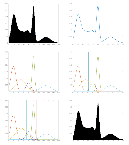
In image processing and computer vision, traditional image segmentation models often assign to one pixel only one exclusive pattern. In fuzzy or soft segmentation, any pattern can have certain "ownership" over any single pixel. If the patterns are Gaussian, fuzzy segmentation naturally results in Gaussian mixtures. Combined with other analytic or geometric tools (e.g., phase transitions over diffusive boundaries), such spatially regularized mixture models could lead to more realistic and computationally efficient segmentation methods.[8]

Point set registration

Probabilistic mixture models such as Gaussian mixture models (GMM) are used to resolve point set registration problems in image processing and computer vision fields. For pair-wise point set registration, one point set is regarded as the centroids of mixture models, and the other point set is regarded as data points (observations). State-of-the-art methods are e.g. coherent point drift (CPD)[9] and Student's t-distribution mixture models (TMM).[10] The result of recent research demonstrate the superiority of hybrid mixture models[11] (e.g. combining Student's t-Distritubtion and Watson distribution/Bingham distribution to model spatial positions and axes orientations separately) compare to CPD and TMM, in terms of inherent robustness, accuracy and discriminative capacity.

Identifiability

Identifiability refers to the existence of a unique characterization for any one of the models in the class (family) being considered. Estimation procedures may not be well-defined and asymptotic theory may not hold if a model is not identifiable.

Example

Let J be the class of all binomial distributions with n = 2. Then a mixture of two members of J would have

${\displaystyle p_{0}=\pi (1-\theta _{1})^{2}+(1-\pi )(1-\theta _{2})^{2}}$

${\displaystyle p_{1}=2\pi \theta _{1}(1-\theta _{1})+2(1-\pi )\theta _{2}(1-\theta _{2})}$

and p₂ = 1 − p₀ − p₁. Clearly, given p₀ and p₁, it is not possible to determine the above mixture model uniquely, as there are three parameters (π, θ₁, θ₂) to be determined.

Definition

Consider a mixture of parametric distributions of the same class. Let

${\displaystyle J=\{f(\cdot$ ;\theta ):\theta \in \Omega \}}

be the class of all component distributions. Then the convex hull K of J defines the class of all finite mixture of distributions in J:

${\displaystyle K=\left\{p(\cdot ):p(\cdot )=\sum _{i=1}^{n}a_{i}f_{i}(\cdot$ ;\theta _{i}),a_{i}>0,\sum _{i=1}^{n}a_{i}=1,f_{i}(\cdot ;\theta _{i})\in J\ \forall i,n\right\}}

K is said to be identifiable if all its members are unique, that is, given two members p and p′ in K, being mixtures of k distributions and k′ distributions respectively in J, we have p = p′ if and only if, first of all, k = k′ and secondly we can reorder the summations such that a_i = a_i′ and ƒ_i = ƒ_i′ for all i.

Parameter estimation and system identification

Parametric mixture models are often used when we know the distribution Y and we can sample from X, but we would like to determine the a_i and θ_i values. Such situations can arise in studies in which we sample from a population that is composed of several distinct subpopulations.

It is common to think of probability mixture modeling as a missing data problem. One way to understand this is to assume that the data points under consideration have "membership" in one of the distributions we are using to model the data. When we start, this membership is unknown, or missing. The job of estimation is to devise appropriate parameters for the model functions we choose, with the connection to the data points being represented as their membership in the individual model distributions.

A variety of approaches to the problem of mixture decomposition have been proposed, many of which focus on maximum likelihood methods such as expectation maximization (EM) or maximum a posteriori estimation (MAP). Generally these methods consider separately the questions of system identification and parameter estimation; methods to determine the number and functional form of components within a mixture are distinguished from methods to estimate the corresponding parameter values. Some notable departures are the graphical methods as outlined in Tarter and Lock[12] and more recently minimum message length (MML) techniques such as Figueiredo and Jain[13] and to some extent the moment matching pattern analysis routines suggested by McWilliam and Loh (2009).[14]

Expectation maximization (EM)

Expectation maximization (EM) is seemingly the most popular technique used to determine the parameters of a mixture with an a priori given number of components. This is a particular way of implementing maximum likelihood estimation for this problem. EM is of particular appeal for finite normal mixtures where closed-form expressions are possible such as in the following iterative algorithm by Dempster et al. (1977)[15]

${\displaystyle w_{s}^{(j+1)}={\frac {1}{N}}\sum _{t=1}^{N}h_{s}^{(j)}(t)}$

${\displaystyle \mu _{s}^{(j+1)}={\frac {\sum _{t=1}^{N}h_{s}^{(j)}(t)x^{(t)}}{\sum _{t=1}^{N}h_{s}^{(j)}(t)}}}$

${\displaystyle \Sigma _{s}^{(j+1)}={\frac {\sum _{t=1}^{N}h_{s}^{(j)}(t)[x^{(t)}-\mu _{s}^{(j+1)}][x^{(t)}-\mu _{s}^{(j+1)}]^{\top }}{\sum _{t=1}^{N}h_{s}^{(j)}(t)}}}$

with the posterior probabilities

${\displaystyle h_{s}^{(j)}(t)={\frac {w_{s}^{(j)}p_{s}(x^{(t)};\mu _{s}^{(j)},\Sigma _{s}^{(j)})}{\sum _{i=1}^{n}w_{i}^{(j)}p_{i}(x^{(t)};\mu _{i}^{(j)},\Sigma _{i}^{(j)})}}.}$

Thus on the basis of the current estimate for the parameters, the conditional probability for a given observation x^(t) being generated from state s is determined for each t = 1, …, N ; N being the sample size. The parameters are then updated such that the new component weights correspond to the average conditional probability and each component mean and covariance is the component specific weighted average of the mean and covariance of the entire sample.

Dempster[15] also showed that each successive EM iteration will not decrease the likelihood, a property not shared by other gradient based maximization techniques. Moreover, EM naturally embeds within it constraints on the probability vector, and for sufficiently large sample sizes positive definiteness of the covariance iterates. This is a key advantage since explicitly constrained methods incur extra computational costs to check and maintain appropriate values. Theoretically EM is a first-order algorithm and as such converges slowly to a fixed-point solution. Redner and Walker (1984) make this point arguing in favour of superlinear and second order Newton and quasi-Newton methods and reporting slow convergence in EM on the basis of their empirical tests. They do concede that convergence in likelihood was rapid even if convergence in the parameter values themselves was not. The relative merits of EM and other algorithms vis-à-vis convergence have been discussed in other literature.[16]

Other common objections to the use of EM are that it has a propensity to spuriously identify local maxima, as well as displaying sensitivity to initial values.[17][18] One may address these problems by evaluating EM at several initial points in the parameter space but this is computationally costly and other approaches, such as the annealing EM method of Udea and Nakano (1998) (in which the initial components are essentially forced to overlap, providing a less heterogeneous basis for initial guesses), may be preferable.

Figueiredo and Jain[13] note that convergence to 'meaningless' parameter values obtained at the boundary (where regularity conditions breakdown, e.g., Ghosh and Sen (1985)) is frequently observed when the number of model components exceeds the optimal/true one. On this basis they suggest a unified approach to estimation and identification in which the initial n is chosen to greatly exceed the expected optimal value. Their optimization routine is constructed via a minimum message length (MML) criterion that effectively eliminates a candidate component if there is insufficient information to support it. In this way it is possible to systematize reductions in n and consider estimation and identification jointly.

The Expectation-maximization algorithm can be used to compute the parameters of a parametric mixture model distribution (the a_i and θ_i). It is an iterative algorithm with two steps: an expectation step and a maximization step. Practical examples of EM and Mixture Modeling are included in the SOCR demonstrations.

The expectation step

With initial guesses for the parameters of our mixture model, "partial membership" of each data point in each constituent distribution is computed by calculating expectation values for the membership variables of each data point. That is, for each data point x_j and distribution Y_i, the membership value y_{i, j} is:

${\displaystyle y_{i,j}={\frac {a_{i}f_{Y}(x_{j};\theta _{i})}{f_{X}(x_{j})}}.}$

The maximization step

With expectation values in hand for group membership, plug-in estimates are recomputed for the distribution parameters.

The mixing coefficients a_i are the means of the membership values over the N data points.

${\displaystyle a_{i}={\frac {1}{N}}\sum _{j=1}^{N}y_{i,j}}$

The component model parameters θ_i are also calculated by expectation maximization using data points x_j that have been weighted using the membership values. For example, if θ is a mean μ

${\displaystyle \mu _{i}={\frac {\sum _{j}y_{i,j}x_{j}}{\sum _{j}y_{i,j}}}.}$

With new estimates for a_i and the θ_i's, the expectation step is repeated to recompute new membership values. The entire procedure is repeated until model parameters converge.

Markov chain Monte Carlo

As an alternative to the EM algorithm, the mixture model parameters can be deduced using posterior sampling as indicated by Bayes' theorem. This is still regarded as an incomplete data problem whereby membership of data points is the missing data. A two-step iterative procedure known as Gibbs sampling can be used.

The previous example of a mixture of two Gaussian distributions can demonstrate how the method works. As before, initial guesses of the parameters for the mixture model are made. Instead of computing partial memberships for each elemental distribution, a membership value for each data point is drawn from a Bernoulli distribution (that is, it will be assigned to either the first or the second Gaussian). The Bernoulli parameter θ is determined for each data point on the basis of one of the constituent distributions. Draws from the distribution generate membership associations for each data point. Plug-in estimators can then be used as in the M step of EM to generate a new set of mixture model parameters, and the binomial draw step repeated.

Moment matching

The method of moment matching is one of the oldest techniques for determining the mixture parameters dating back to Karl Pearson's seminal work of 1894. In this approach the parameters of the mixture are determined such that the composite distribution has moments matching some given value. In many instances extraction of solutions to the moment equations may present non-trivial algebraic or computational problems. Moreover, numerical analysis by Day[19] has indicated that such methods may be inefficient compared to EM. Nonetheless there has been renewed interest in this method, e.g., Craigmile and Titterington (1998) and Wang.[20]

McWilliam and Loh (2009) consider the characterisation of a hyper-cuboid normal mixture copula in large dimensional systems for which EM would be computationally prohibitive. Here a pattern analysis routine is used to generate multivariate tail-dependencies consistent with a set of univariate and (in some sense) bivariate moments. The performance of this method is then evaluated using equity log-return data with Kolmogorov–Smirnov test statistics suggesting a good descriptive fit.

Spectral method

Some problems in mixture model estimation can be solved using spectral methods. In particular it becomes useful if data points x_i are points in high-dimensional real space, and the hidden distributions are known to be log-concave (such as Gaussian distribution or Exponential distribution).

Spectral methods of learning mixture models are based on the use of Singular Value Decomposition of a matrix which contains data points. The idea is to consider the top k singular vectors, where k is the number of distributions to be learned. The projection of each data point to a linear subspace spanned by those vectors groups points originating from the same distribution very close together, while points from different distributions stay far apart.

One distinctive feature of the spectral method is that it allows us to prove that if distributions satisfy certain separation condition (e.g., not too close), then the estimated mixture will be very close to the true one with high probability.

Graphical Methods

Tarter and Lock[12] describe a graphical approach to mixture identification in which a kernel function is applied to an empirical frequency plot so to reduce intra-component variance. In this way one may more readily identify components having differing means. While this λ-method does not require prior knowledge of the number or functional form of the components its success does rely on the choice of the kernel parameters which to some extent implicitly embeds assumptions about the component structure.

Other methods

Some of them can even probably learn mixtures of heavy-tailed distributions including those with infinite variance (see links to papers below). In this setting, EM based methods would not work, since the Expectation step would diverge due to presence of outliers.

A simulation

To simulate a sample of size N that is from a mixture of distributions F_i, i=1 to n, with probabilities p_i (sum= p_i = 1):

1. Generate N random numbers from a categorical distribution of size n and probabilities p_i for i= 1= to n. These tell you which of the F_i each of the N values will come from. Denote by m_i the quantity of random numbers assigned to the i^th category.
2. For each i, generate m_i random numbers from the F_i distribution.

Extensions

In a Bayesian setting, additional levels can be added to the graphical model defining the mixture model. For example, in the common latent Dirichlet allocation topic model, the observations are sets of words drawn from D different documents and the K mixture components represent topics that are shared across documents. Each document has a different set of mixture weights, which specify the topics prevalent in that document. All sets of mixture weights share common hyperparameters.

A very common extension is to connect the latent variables defining the mixture component identities into a Markov chain, instead of assuming that they are independent identically distributed random variables. The resulting model is termed a hidden Markov model and is one of the most common sequential hierarchical models. Numerous extensions of hidden Markov models have been developed; see the resulting article for more information.

History

Mixture distributions and the problem of mixture decomposition, that is the identification of its constituent components and the parameters thereof, has been cited in the literature as far back as 1846 (Quetelet in McLachlan, [17] 2000) although common reference is made to the work of Karl Pearson (1894)[21] as the first author to explicitly address the decomposition problem in characterising non-normal attributes of forehead to body length ratios in female shore crab populations. The motivation for this work was provided by the zoologist Walter Frank Raphael Weldon who had speculated in 1893 (in Tarter and Lock[12]) that asymmetry in the histogram of these ratios could signal evolutionary divergence. Pearson's approach was to fit a univariate mixture of two normals to the data by choosing the five parameters of the mixture such that the empirical moments matched that of the model.

While his work was successful in identifying two potentially distinct sub-populations and in demonstrating the flexibility of mixtures as a moment matching tool, the formulation required the solution of a 9th degree (nonic) polynomial which at the time posed a significant computational challenge.

Subsequent works focused on addressing these problems, but it was not until the advent of the modern computer and the popularisation of Maximum Likelihood (MLE) parameterisation techniques that research really took off.[22] Since that time there has been a vast body of research on the subject spanning areas such as fisheries research, agriculture, botany, economics, medicine, genetics, psychology, palaeontology, electrophoresis, finance, geology and zoology.[23]

See also

Mixture

• Mixture density
• Mixture (probability)
• Flexible Mixture Model (FMM)

Hierarchical models

• Graphical model
• Hierarchical Bayes model

Outlier detection

• RANSAC

References

1. Sotirios P. Chatzis, Dimitrios I. Kosmopoulos, Theodora A. Varvarigou, "Signal Modeling and Classification Using a Robust Latent Space Model Based on t Distributions," IEEE Transactions on Signal Processing, vol. 56, no. 3, pp. 949–963, March 2008.
2. Yu, Guoshen (2012). "Solving Inverse Problems with Piecewise Linear Estimators: From Gaussian Mixture Models to Structured Sparsity". IEEE Transactions on Image Processing. 21 (5): 2481–2499. arXiv:1006.3056. Bibcode:2012ITIP...21.2481G. doi:10.1109/tip.2011.2176743. PMID 22180506.
3. Dinov, ID. "Expectation Maximization and Mixture Modeling Tutorial". California Digital Library, Statistics Online Computational Resource, Paper EM_MM, http://repositories.cdlib.org/socr/EM_MM, December 9, 2008
4. Bishop, Christopher (2006). Pattern recognition and machine learning. New York: Springer. ISBN 978-0-387-31073-2.
5. Spall, J. C. and Maryak, J. L. (1992). "A feasible Bayesian estimator of quantiles for projectile accuracy from non-i.i.d. data." Journal of the American Statistical Association, vol. 87 (419), pp. 676–681. JSTOR 2290205
6. Amruthnath, Nagdev; Gupta, Tarun (2018-02-02). Fault Class Prediction in Unsupervised Learning using Model-Based Clustering Approach. Unpublished. doi:10.13140/rg.2.2.22085.14563.
7. Amruthnath, Nagdev; Gupta, Tarun (2018-02-01). A Research Study on Unsupervised Machine Learning Algorithms for Fault Detection in Predictive Maintenance. Unpublished. doi:10.13140/rg.2.2.28822.24648.
8. Shen, Jianhong (Jackie) (2006). "A stochastic-variational model for soft Mumford-Shah segmentation". International Journal of Biomedical Imaging. 2006: 2–16. Bibcode:2006IJBI.200649515H. doi:10.1155/IJBI/2006/92329. PMC 2324060. PMID 23165059.
9. Myronenko, Andriy; Song, Xubo (2010). "Point set registration: Coherent point drift". IEEE Trans. Pattern Anal. Mach. Intell. 32 (12): 2262–2275. arXiv:0905.2635. doi:10.1109/TPAMI.2010.46. PMID 20975122.
10. Ravikumar, Nishant; Gooya, Ali; Cimen, Serkan; Frangi, Alexjandro; Taylor, Zeike (2018). "Group-wise similarity registration of point sets using Student's t-mixture model for statistical shape models". Med. Image. Anal. 44: 156–176. doi:10.1016/j.media.2017.11.012. PMID 29248842.
11. Bayer, Siming; Ravikumar, Nishant; Strumia, Maddalena; Tong, Xiaoguang; Gao, Ying; Ostermeier, Martin; Fahrig, Rebecca; Maier, Andreas (2018). "Intraoperative brain shift compensation using a hybrid mixture model". Medical Image Computing and Computer Assisted Intervention – MICCAI 2018. Granada, Spain: Springer, Cham. pp. 116–124. doi:10.1007/978-3-030-00937-3_14.
12. Tarter, Michael E. (1993), Model Free Curve Estimation, Chapman and Hall
13. Figueiredo, M.A.T.; Jain, A.K. (March 2002). "Unsupervised Learning of Finite Mixture Models". IEEE Transactions on Pattern Analysis and Machine Intelligence. 24 (3): 381–396. CiteSeerX 10.1.1.362.9811. doi:10.1109/34.990138.
14. McWilliam, N.; Loh, K. (2008), Incorporating Multidimensional Tail-Dependencies in the Valuation of Credit Derivatives (Working Paper)
15. Dempster, A.P.; Laird, N.M.; Rubin, D.B. (1977). "Maximum Likelihood from Incomplete Data via the EM Algorithm". Journal of the Royal Statistical Society, Series B. 39 (1): 1–38. CiteSeerX 10.1.1.163.7580. JSTOR 2984875.
16. Xu, L.; Jordan, M.I. (January 1996). "On Convergence Properties of the EM Algorithm for Gaussian Mixtures". Neural Computation. 8 (1): 129–151. doi:10.1162/neco.1996.8.1.129. hdl:10338.dmlcz/135225.
17. McLachlan, G.J. (2000), Finite Mixture Models, Wiley
18. Botev, Z.I.; Kroese, D.P. (2004). Global likelihood optimization via the cross-entropy method with an application to mixture models. Proceedings of the 2004 Winter Simulation Conference. 1. p. 517. CiteSeerX 10.1.1.331.2319. doi:10.1109/WSC.2004.1371358. ISBN 978-0-7803-8786-7.
19. Day, N. E. (1969). "Estimating the Components of a Mixture of Normal Distributions". Biometrika. 56 (3): 463–474. doi:10.2307/2334652. JSTOR 2334652.
20. Wang, J. (2001), "Generating daily changes in market variables using a multivariate mixture of normal distributions", Proceedings of the 33rd Winter Conference on Simulation: 283–289
21. Améndola, Carlos; et al. (2015). "Moment varieties of Gaussian mixtures". Journal of Algebraic Statistics. 7. arXiv:1510.04654. Bibcode:2015arXiv151004654A. doi:10.18409/jas.v7i1.42.
22. McLachlan, G.J.; Basford, K.E. (1988), "Mixture Models: inference and applications to clustering", Statistics: Textbooks and Monographs, Bibcode:1988mmia.book.....M
23. Titterington, Smith & Makov 1985

Further reading

Books on mixture models

• Everitt, B.S.; Hand, D.J. (1981). Finite mixture distributions. Chapman & Hall. ISBN 978-0-412-22420-1.
• Lindsay, B. G. (1995). Mixture Models: Theory, Geometry, and Applications. NSF-CBMS Regional Conference Series in Probability and Statistics. 5. Hayward: Institute of Mathematical Statistics.
• Marin, J.M.; Mengersen, K.; Robert, C.P. (2011). "Bayesian modelling and inference on mixtures of distributions" (PDF). In Dey, D.; Rao, C.R. (eds.). Essential Bayesian models. Handbook of statistics: Bayesian thinking - modeling and computation. 25. Elsevier. ISBN 9780444537324.
• McLachlan, G.J.; Peel, D. (2000). Finite Mixture Models. Wiley. ISBN 978-0-471-00626-8.
• Press, WH; Teukolsky, SA; Vetterling, WT; Flannery, BP (2007). "Section 16.1. Gaussian Mixture Models and k-Means Clustering". Numerical Recipes: The Art of Scientific Computing (3rd ed.). New York: Cambridge University Press. ISBN 978-0-521-88068-8.
• Titterington, D.; Smith, A.; Makov, U. (1985). Statistical Analysis of Finite Mixture Distributions. Wiley. ISBN 978-0-471-90763-3.CS1 maint: ref=harv (link)

Application of Gaussian mixture models

1. Reynolds, D.A.; Rose, R.C. (January 1995). "Robust text-independent speaker identification using Gaussian mixture speaker models". IEEE Transactions on Speech and Audio Processing. 3 (1): 72–83. doi:10.1109/89.365379.
2. Permuter, H.; Francos, J.; Jermyn, I.H. (2003). Gaussian mixture models of texture and colour for image database retrieval. IEEE International Conference on Acoustics, Speech, and Signal Processing, 2003. Proceedings (ICASSP '03). doi:10.1109/ICASSP.2003.1199538.
   • Permuter, Haim; Francos, Joseph; Jermyn, Ian (2006). "A study of Gaussian mixture models of color and texture features for image classification and segmentation" (PDF). Pattern Recognition. 39 (4): 695–706. doi:10.1016/j.patcog.2005.10.028.
3. Lemke, Wolfgang (2005). Term Structure Modeling and Estimation in a State Space Framework. Springer Verlag. ISBN 978-3-540-28342-3.
4. Brigo, Damiano; Mercurio, Fabio (2001). Displaced and Mixture Diffusions for Analytically-Tractable Smile Models. Mathematical Finance – Bachelier Congress 2000. Proceedings. Springer Verlag.
5. Brigo, Damiano; Mercurio, Fabio (June 2002). "Lognormal-mixture dynamics and calibration to market volatility smiles". International Journal of Theoretical and Applied Finance. 5 (4): 427. CiteSeerX 10.1.1.210.4165. doi:10.1142/S0219024902001511.
6. Spall, J. C.; Maryak, J. L. (1992). "A feasible Bayesian estimator of quantiles for projectile accuracy from non-i.i.d. data". Journal of the American Statistical Association. 87 (419): 676–681. doi:10.1080/01621459.1992.10475269. JSTOR 2290205.
7. Alexander, Carol (December 2004). "Normal mixture diffusion with uncertain volatility: Modelling short- and long-term smile effects" (PDF). Journal of Banking & Finance. 28 (12): 2957–80. doi:10.1016/j.jbankfin.2003.10.017.
8. Stylianou, Yannis; Pantazis, Yannis; Calderero, Felipe; Larroy, Pedro; Severin, Francois; Schimke, Sascha; Bonal, Rolando; Matta, Federico; Valsamakis, Athanasios (2005). GMM-Based Multimodal Biometric Verification (PDF).
9. Chen, J.; Adebomi, 0.E.; Olusayo, O.S.; Kulesza, W. (2010). The Evaluation of the Gaussian Mixture Probability Hypothesis Density approach for multi-target tracking. IEEE International Conference on Imaging Systems and Techniques, 2010. doi:10.1109/IST.2010.5548541.

External links

• Nielsen, Frank (23 March 2012). k-MLE: A fast algorithm for learning statistical mixture models. 2012 IEEE International Conference on Acoustics, Speech and Signal Processing (ICASSP). pp. 869–872. arXiv:1203.5181. Bibcode:2012arXiv1203.5181N. doi:10.1109/ICASSP.2012.6288022. ISBN 978-1-4673-0046-9.
• The SOCR demonstrations of EM and Mixture Modeling
• Mixture modelling page (and the Snob program for Minimum Message Length (MML) applied to finite mixture models), maintained by D.L. Dowe.
• PyMix – Python Mixture Package, algorithms and data structures for a broad variety of mixture model based data mining applications in Python
• sklearn.mixture – A Python package for learning Gaussian Mixture Models (and sampling from them), previously packaged with SciPy and now packaged as a SciKit
• GMM.m Matlab code for GMM Implementation
• GPUmix C++ implementation of Bayesian Mixture Models using EM and MCMC with 100x speed acceleration using GPGPU.
• Matlab code for GMM Implementation using EM algorithm
• jMEF: A Java open source library for learning and processing mixtures of exponential families (using duality with Bregman divergences). Includes a Matlab wrapper.
• Very Fast and clean C implementation of the Expectation Maximization (EM) algorithm for estimating Gaussian Mixture Models (GMMs).
• mclust is an R package for mixture modeling.
• dpgmm Pure Python Dirichlet process Gaussian mixture model implementation (variational).
• Gaussian Mixture Models Blog post on Gaussian Mixture Models trained via Expectation Maximization, with an implementation in Python.