Free electron model

In solid-state physics, the free electron model is a simple model for the behaviour of charge carriers in a metallic solid. It was developed in 1927,[1] principally by Arnold Sommerfeld, who combined the classical Drude model with quantum mechanical Fermi–Dirac statistics and hence it is also known as the Drude–Sommerfeld model.

This article is about the solid-state model for metals. For the model of a free electron gas, see Fermi gas.

Given its simplicity, it is surprisingly successful in explaining many experimental phenomena, especially

• the Wiedemann–Franz law which relates electrical conductivity and thermal conductivity;
• the temperature dependence of the electron heat capacity;
• the shape of the electronic density of states;
• the range of binding energy values;
• electrical conductivities;
• the Seebeck coefficient of the thermoelectric effect;
• thermal electron emission and field electron emission from bulk metals.

The free electron model solved many of the inconsistencies related to the Drude model and gave insight into several other properties of metals. The free electron model considers that metals are composed of a quantum electron gas where ions play almost no role. The model can be very predictive when applied to alkali and noble metals.

Ideas and assumptions

In the free electron model four main assumptions are taken into account:

• Free electron approximation: The interaction between the ions and the valence electrons is mostly neglected, except in boundary conditions. The ions only keep the charge neutrality in the metal. Unlike in the Drude model, the ions are not necessarily the source of collisions.
• Independent electron approximation: The interactions between electrons are ignored. The electrostatic fields in metals are weak because of the screening effect.
• Relaxation-time approximation: There is some unknown scattering mechanism such that the electron probability of collision is inversely proportional to the relaxation time ${\displaystyle \tau }$, which represents the average time between collisions. The collisions do not depend on the electronic configuration.
• Pauli exclusion principle: Each quantum state of the system can only be occupied by a single electron. This restriction of available electron states is taken into account by Fermi–Dirac statistics (see also Fermi gas). Main predictions of the free-electron model are derived by the Sommerfeld expansion of the Fermi–Dirac occupancy for energies around the Fermi level.

The name of the model comes from the first two assumptions, as each electron can be treated as free particle with a respective quadratic relation between energy and momentum.

The crystal lattice is not explicitly taken into account in the free electron model, but a quantum-mechanical justification was given a year later (1928) by Bloch's theorem: an unbound electron moves in a periodic potential as a free electron in vacuum, except for the electron mass m_e becoming an effective mass m* which may deviate considerably from m_e (one can even use negative effective mass to describe conduction by electron holes). Effective masses can be derived from band structure computations that were not originally taken into account in the free electron model.

From the Drude model

Main article: Drude model

Many physical properties follow directly from the Drude model, as some equations do not depend on the statistical distribution of the particles. Taking the classical velocity distribution of an ideal gas or the velocity distribution of a Fermi gas only changes the results related to the speed of the electrons.

Mainly, the free electron model and the Drude model predict the same DC electrical conductivity σ for Ohm's law, that is

${\displaystyle \mathbf {J} =\sigma \mathbf {E} \quad }$ with ${\displaystyle \quad \sigma ={\frac {ne^{2}\tau }{m_{e}}},}$

where ${\displaystyle \mathbf {J} }$ is the current density, ${\displaystyle \mathbf {E} }$ is the external electric field, ${\displaystyle n}$ is the electronic density (number of electrons/volume), ${\displaystyle \tau }$ is the mean free time and ${\displaystyle e}$ is the electron electric charge.

Other quantities that remain the same under the free electron model as under Drude's are the AC susceptibility, the plasma frequency, the magnetoresistance, and the Hall coefficient related to the Hall effect.

Properties of an electron gas

Main article: Fermi gas

Many properties of the free electron model follow directly from equations related to the Fermi gas, as the independent electron approximation leads to an ensemble of non-interacting electrons. For a three-dimensional electron gas we can define the Fermi energy as

${\displaystyle E_{\rm {F}}={\frac {\hbar ^{2}}{2m_{e}}}\left(3\pi ^{2}n\right)^{\frac {2}{3}},}$

where ${\displaystyle \hbar }$ is the reduced Planck constant. The Fermi energy defines the energy of the highest energy electron at zero temperature. For metals the Fermi energy is in the order of units of electronvolts above the free electron band minimum energy.[2]

In three dimensions, the density of states of a gas of fermions is proportional to the square root of the kinetic energy of the particles.

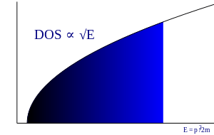
Density of states

The 3D density of states (number of energy states, per energy per volume) of a non-interacting electron gas is given by:

${\displaystyle g(E)={\frac {m_{e}}{\pi ^{2}\hbar ^{3}}}{\sqrt {2m_{e}E}}={\frac {3}{2}}{\frac {n}{E_{\rm {F}}}}{\sqrt {\frac {E}{E_{\rm {F}}}}},}$

where ${\textstyle E\geq 0}$ is the energy of a given electron. This formula takes into account the spin degeneracy but does not consider a possible energy shift due to the bottom of the conduction band. For 2D the density of states is constant and for 1D is inversely proportional to the square root of the electron energy.

Fermi level

The chemical potential ${\displaystyle \mu }$ of electrons in a solid is also known as the Fermi level and, like the related Fermi energy, often denoted ${\displaystyle E_{\rm {F}}}$. The Sommerfeld expansion can be used to calculate the Fermi level (${\displaystyle T>0}$) at higher temperatures as:

${\displaystyle E_{\rm {F}}(T)=E_{\rm {F}}(T=0)\left[1-{\frac {\pi ^{2}}{12}}\left({\frac {T}{T_{\rm {F}}}}\right)^{2}-{\frac {\pi ^{4}}{80}}\left({\frac {T}{T_{\rm {F}}}}\right)^{4}+\cdots \right],}$

where ${\displaystyle T}$ is the temperature and we define ${\textstyle T_{\rm {F}}=E_{\rm {F}}/k_{\rm {B}}}$ as the Fermi temperature (${\displaystyle k_{\rm {B}}}$ is Boltzmann constant). The perturbative approach is justified as the Fermi temperature is usually of about 10⁵ K for a metal, hence at room temperature or lower the Fermi energy ${\displaystyle E_{\rm {F}}(T=0)}$ and the chemical potential ${\displaystyle E_{\rm {F}}(T>0)}$ are practically equivalent.

Compressibility of metals and degeneracy pressure

The total energy per unit volume (at ${\textstyle T=0}$) can also be calculated by integrating over the phase space of the system, we obtain

${\displaystyle u(0)={\frac {3}{5}}nE_{\rm {F}},}$

which does not depend on temperature. Compare with the energy per electron of an ideal gas: ${\textstyle {\frac {3}{2}}k_{\rm {B}}T}$, which is null at zero temperature. For an ideal gas to have the same energy as the electron gas, the temperatures would need to be of the order of the Fermi temperature. Thermodynamically, this energy of the electron gas corresponds to a zero-temperature pressure given by

${\displaystyle P=-\left({\frac {\partial U}{\partial V}}\right)_{T,\mu }={\frac {2}{3}}u(0),}$

where ${\textstyle V}$ is the volume and ${\textstyle U(T)=u(T)V}$ is the total energy, the derivative performed at temperature and chemical potential constant. This pressure is called the electron degeneracy pressure and does not come from repulsion or motion of the electrons but from the restriction that no more than two electrons (due to the two values of spin) can occupy the same energy level. This pressure defines the compressibility or bulk modulus of the metal

${\displaystyle B=-V\left({\frac {\partial P}{\partial V}}\right)_{T,\mu }={\frac {5}{3}}P={\frac {2}{3}}nE_{\rm {F}}.}$

This expression gives the right order of magnitude for the bulk modulus for alkali metals and noble metals, which show that this pressure is as important as other effects inside the metal. For other metals the crystalline structure has to be taken into account.

Additional predictions

Heat capacity

Further information: Electron heat capacity

One open problem in solid-state physics before the arrival of the free electron model was related to the low heat capacity of metals. Even when the Drude model was a good approximation for the Lorenz number of the Wiedemann–Franz law, the classical argument is based on the idea that the volumetric heat capacity of an ideal gas is

${\displaystyle c_{V}^{\text{Drude}}={\frac {3}{2}}nk_{\rm {B}}}$.

If this was the case, the heat capacity of a metal could be much higher due to this electronic contribution. Nevertheless, such a large heat capacity was never measured, raising suspicions about the argument. By using Sommerfeld's expansion one can obtain corrections of the energy density at finite temperature and obtain the volumetric heat capacity of an electron gas, given by:

${\displaystyle c_{V}=\left({\frac {\partial u}{\partial T}}\right)_{n}={\frac {\pi ^{2}}{2}}{\frac {T}{T_{\rm {F}}}}nk_{\rm {B}}}$,

where the prefactor to ${\displaystyle nk_{B}}$is considerably smaller than the 3/2 found in ${\textstyle c_{V}^{\text{Drude}}}$, about 100 times smaller at room temperature and much smaller at lower ${\textstyle T}$. The good estimation of the Lorenz number in the Drude model was a result of the classical mean velocity of electron being about 100 larger than the quantum version, compensating the large value of the classical heat capacity. The free electron model calculation of the Lorenz factor is about twice the value of Drude's and its closer to the experimental value. With this heat capacity the free electron model is also able to predict the right order of magnitude and temperature dependence at low T for the Seebeck coefficient of the thermoelectric effect.

Evidently, the electronic contribution alone does not predict the Dulong–Petit law, i.e. the observation that the heat capacity of a metal is constant at high temperatures. The free electron model can be improved in this sense by adding the lattice vibrations contribution. Two famous schemes to include the lattice into the problem are the Einstein solid model and Debye model. With the addition of the later, the volumetric heat capacity of a metal at low temperatures can be more precisely written in the form,

${\displaystyle c_{V}\approx \gamma T+AT^{3}}$,

where ${\displaystyle \gamma }$ and ${\displaystyle A}$ are constants related to the material. The linear term comes from the electronic contribution while the cubic term comes from Debye model. At high temperature this expression is no longer correct, the electronic heat capacity can be neglected, and the total heat capacity of the metal tends to a constant.

Mean free path

Notice that without the relaxation time approximation, there is no reason for the electrons to deflect their motion, as there are no interactions, thus the mean free path should be infinite. The Drude model considered the mean free path of electrons to be close to the distance between ions in the material, implying the earlier conclusion that the diffusive motion of the electrons was due to collisions with the ions. The mean free paths in the free electron model are instead given by ${\textstyle \lambda =v_{\rm {F}}\tau }$ (where ${\textstyle v_{\rm {F}}={\sqrt {2E_{\rm {F}}/m_{e}}}}$ is the Fermi speed) and are in the order of hundreds of ångströms, at least one order of magnitude larger than any possible classical calculation. The mean free path is then not a result of electron–ion collisions but instead is related to imperfections in the material, either due to defects and impurities in the metal, or due to thermal fluctuations.[3]

Inaccuracies and extensions

The free electron model presents several inadequacies that are contradicted by experimental observation. We list some inaccuracies below:

Temperature dependence

The free electron model presents several physical quantities that have the wrong temperature dependence, or no dependence at all like the electrical conductivity. The thermal conductivity and specific heat are well predicted for alkali metals at low temperatures, but fails to predict high temperature behaviour coming from ion motion and phonon scattering.

Hall effect and magnetoresistance

The Hall coefficient has a constant value R_H = –1/(ne) in Drude's model and in the free electron model. This value is independent of temperature and the strength of the magnetic field. The Hall coefficient is actually dependent on the band structure and the difference with the model can be quite dramatic when studying elements like magnesium and aluminium that have a strong magnetic field dependence. The free electron model also predicts that the traverse magnetoresistance, the resistance in the direction of the current, does not depend on the strength of the field. In almost all the cases it does.

Directional

The conductivity of some metals can depend of the orientation of the sample with respect to the electric field. Sometimes even the electrical current is not parallel to the field. This possibility is not described because the model does not integrate the crystallinity of metals, i.e. the existence of a periodic lattice of ions.

Diversity in the conductivity

Not all materials are electrical conductors, some do not conduct electricity very well (insulators), some can conduct when impurities are added like semiconductors. Semimetals, with narrow conduction bands also exist. This diversity is not predicted by the model and can only by explained by analysing the valence and conduction bands. Additionally, electrons are not the only charge carriers in a metal, electron vacancies or holes can be seen as quasiparticles carrying positive electric charge. Conduction of holes leads to an opposite sign for the Hall and Seebeck coefficients predicted by the model.

Other inadequacies are present in the Wiedemann–Franz law at intermediate temperatures and the frequency-dependence of metals in the optical spectrum.

More exact values for the electrical conductivity and Wiedemann–Franz law can be obtained by softening the relaxation-time approximation by appealing to the Boltzmann transport equations or the Kubo formula.

Spin is mostly neglected in the free electron model and its consequences can lead to emergent magnetic phenomena like Pauli paramagnetism and ferromagnetism.

An immediate continuation to the free electron model can be obtained by assuming the empty lattice approximation, which forms the basis of the band structure model known as the nearly free electron model.

Adding repulsive interactions between electrons does not change very much the picture presented here. Lev Landau showed that a Fermi gas under repulsive interactions, can be seen as a gas of equivalent quasiparticles that slightly modify the properties of the metal. Landau's model is now known as the Fermi liquid theory. More exotic phenomena like superconductivity, where interactions can be attractive, require a more refined theory.

See also

• Bloch wave
• Electronic entropy
• Tight binding
• Two-dimensional electron gas
• Bose–Einstein statistics
• Fermi surface
• White dwarf

References

1. Sommerfeld, Arnold (1928-01-01). "Zur Elektronentheorie der Metalle auf Grund der Fermischen Statistik". Zeitschrift für Physik (in German). 47 (1–2): 1–32. Bibcode:1928ZPhy...47....1S. doi:10.1007/bf01391052. ISSN 0044-3328.
2. Nave, Rod. "Fermi Energies, Fermi Temperatures, and Fermi Velocities". HyperPhysics. Retrieved 2018-03-21.
3. Tsymbal, Evgeny (2008). "Electronic Transport" (PDF). University of Nebraska-Lincoln. Retrieved 2018-04-21.

General

• Kittel, Charles (1953). Introduction to Solid State Physics. University of Michigan: Wiley.
• Ashcroft, Neil; Mermin, N. David (1976). Solid State Physics. New York: Holt, Rinehart and Winston. ISBN 978-0-03-083993-1.
• Sommerfeld, Arnold; Bethe, Hans (1933). Elektronentheorie der Metalle. Berlin Heidelberg: Springer Verlag. ISBN 978-3642950025.