Erdős–Rényi model

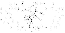
In the mathematical field of graph theory, the Erdős–Rényi model is either of two closely related models for generating random graphs. They are named after mathematicians Paul Erdős and Alfréd Rényi, who first introduced one of the models in 1959,[1][2] while Edgar Gilbert introduced the other model contemporaneously and independently of Erdős and Rényi.[3] In the model of Erdős and Rényi, all graphs on a fixed vertex set with a fixed number of edges are equally likely; in the model introduced by Gilbert, each edge has a fixed probability of being present or absent, independently of the other edges. These models can be used in the probabilistic method to prove the existence of graphs satisfying various properties, or to provide a rigorous definition of what it means for a property to hold for almost all graphs.

Definition

There are two closely related variants of the Erdős–Rényi random graph model.

A graph generated by the binomial model of Erdős and Rényi (p = 0.01)

In the G(n, M) model, a graph is chosen uniformly at random from the collection of all graphs which have n nodes and M edges. For example, in the G(3, 2) model, each of the three possible graphs on three vertices and two edges are included with probability 1/3.
In the G(n, p) model, a graph is constructed by connecting nodes randomly. Each edge is included in the graph with probability p independent from every other edge. Equivalently, all graphs with n nodes and M edges have equal probability of

p^{M}(1-p)^{{n \choose 2}-M}.

The parameter p in this model can be thought of as a weighting function; as p increases from 0 to 1, the model becomes more and more likely to include graphs with more edges and less and less likely to include graphs with fewer edges. In particular, the case p = 0.5 corresponds to the case where all

2^{\binom {n}{2}}

graphs on n vertices are chosen with equal probability.

The behavior of random graphs are often studied in the case where n, the number of vertices, tends to infinity. Although p and M can be fixed in this case, they can also be functions depending on n. For example, the statement

Almost every graph in G(n, 2ln(n)/n) is connected.

means

As n tends to infinity, the probability that a graph on n vertices with edge probability 2ln(n)/n is connected, tends to 1.

Comparison between the two models

The expected number of edges in G(n, p) is ${\tbinom {n}{2}}p$ , and by the law of large numbers any graph in G(n, p) will almost surely have approximately this many edges (provided the expected number of edges tends to infinity). Therefore, a rough heuristic is that if pn² → ∞, then G(n,p) should behave similarly to G(n, M) with $M={\tbinom {n}{2}}p$ as n increases.

For many graph properties, this is the case. If P is any graph property which is monotone with respect to the subgraph ordering (meaning that if A is a subgraph of B and A satisfies P, then B will satisfy P as well), then the statements "P holds for almost all graphs in G(n, p)" and "P holds for almost all graphs in $G(n,{\tbinom {n}{2}}p)$ " are equivalent (provided pn² → ∞). For example, this holds if P is the property of being connected, or if P is the property of containing a Hamiltonian cycle. However, this will not necessarily hold for non-monotone properties (e.g. the property of having an even number of edges).

In practice, the G(n, p) model is the one more commonly used today, in part due to the ease of analysis allowed by the independence of the edges.

Properties of G(n, p)

With the notation above, a graph in G(n, p) has on average ${\tbinom {n}{2}}p$ edges. The distribution of the degree of any particular vertex is binomial:[4]

P(\deg(v)=k)={n-1 \choose k}p^{k}(1-p)^{n-1-k},

where n is the total number of vertices in the graph. Since

P(\deg(v)=k)\to {\frac {(np)^{k}\mathrm {e} ^{-np}}{k!}}\quad {\text{ as }}n\to \infty {\text{ and }}np={\text{constant}},

this distribution is Poisson for large n and np = const.

In a 1960 paper, Erdős and Rényi[5] described the behavior of G(n, p) very precisely for various values of p. Their results included that:

If np < 1, then a graph in G(n, p) will almost surely have no connected components of size larger than O(log(n)).
If np = 1, then a graph in G(n, p) will almost surely have a largest component whose size is of order n^2/3.
If np → c > 1, where c is a constant, then a graph in G(n, p) will almost surely have a unique giant component containing a positive fraction of the vertices. No other component will contain more than O(log(n)) vertices.
If $p<{\tfrac {(1-\varepsilon )\ln n}{n}}$ , then a graph in G(n, p) will almost surely contain isolated vertices, and thus be disconnected.
If $p>{\tfrac {(1+\varepsilon )\ln n}{n}}$ , then a graph in G(n, p) will almost surely be connected.

Thus ${\tfrac {\ln n}{n}}$ is a sharp threshold for the connectedness of G(n, p).

Further properties of the graph can be described almost precisely as n tends to infinity. For example, there is a k(n) (approximately equal to 2log₂(n)) such that the largest clique in G(n, 0.5) has almost surely either size k(n) or k(n) + 1.[6]

Thus, even though finding the size of the largest clique in a graph is NP-complete, the size of the largest clique in a "typical" graph (according to this model) is very well understood.

Edge-dual graphs of Erdos-Renyi graphs are graphs with nearly the same degree distribution, but with degree correlations and a significantly higher clustering coefficient.[7]

Relation to percolation

In percolation theory one examines a finite or infinite graph and removes edges (or links) randomly. Thus the Erdős–Rényi process is in fact unweighted link percolation on the complete graph. (One refers to percolation in which nodes and/or links are removed with heterogeneous weights as weighted percolation). As percolation theory has much of its roots in physics, much of the research done was on the lattices in Euclidean spaces. The transition at np = 1 from giant component to small component has analogs for these graphs, but for lattices the transition point is difficult to determine. Physicists often refer to study of the complete graph as a mean field theory. Thus the Erdős–Rényi process is the mean-field case of percolation.

Some significant work was also done on percolation on random graphs. From a physicist's point of view this would still be a mean-field model, so the justification of the research is often formulated in terms of the robustness of the graph, viewed as a communication network. Given a random graph of n ≫ 1 nodes with an average degree <k>. Remove randomly a fraction 1 − p′ of nodes and leave only a fraction p′ from the network. There exists a critical percolation threshold $p'_{c}={\tfrac {1}{\langle k\rangle }}$ below which the network becomes fragmented while above $p'_{c}$ a giant connected component of order n exists. The relative size of the giant component, P_∞, is given by[5][1][2][8]

P_{\infty }=p'[1-\exp(-\langle k\rangle P_{\infty })].\,

Caveats

Both of the two major assumptions of the G(n, p) model (that edges are independent and that each edge is equally likely) may be inappropriate for modeling certain real-life phenomena. Erdős–Rényi graphs have low clustering, unlike many social networks. Some modeling alternatives include Barabási–Albert model and Watts and Strogatz model. These alternative models are not percolation processes, but instead represent a growth and rewiring model, respectively. A model for interacting Erdős–Rényi networks was developed recently by Buldyrev et al.[9]

History

The G(n, p) model was first introduced by Edgar Gilbert in a 1959 paper studying the connectivity threshold mentioned above.[3] The G(n, M) model was introduced by Erdős and Rényi in their 1959 paper. As with Gilbert, their first investigations were as to the connectivity of G(n, M), with the more detailed analysis following in 1960.

gollark: Yes, you can use my segfault fixer if that happens.

gollark: Doesn't it just segfault at some point?

gollark: It was more elegance™ to just make it able to do tail-call optimization.

gollark: I actually stole this particular quicksort from a r/haskell post talking about it.

gollark: ```lisp (let (partition_rec xs pred acc) (cond ((= xs '()) acc) (true (partition_rec (tail xs) pred (cond ((pred (head xs)) (list (cons (head xs) (head acc)) (snd acc))) (true (list (head acc) (cons (head xs) (snd acc)))) ))) )) (let (qsort xs cont) (cond ((= xs '()) (cont '())) (true (do (let h (head xs)) (let t (tail xs)) (let part_result (partition_rec t (lambda (x) (< x h)) '(() ()))) (qsort (head part_result) (lambda (ls) (qsort (snd part_result) (lambda (rs) (cont (+ ls (list h) rs)))))) )) ))```These all have to be done tail recursively or it could overflow.

References

Erdős, P.; Rényi, A. (1959). "On Random Graphs. I" (PDF). Publicationes Mathematicae. 6: 290–297.
Bollobás, B. (2001). Random Graphs (2nd ed.). Cambridge University Press. ISBN 0-521-79722-5.
Gilbert, E.N. (1959). "Random Graphs". Annals of Mathematical Statistics. 30 (4): 1141–1144. doi:10.1214/aoms/1177706098.
Newman, Mark. E. J.; Strogatz, S. H.; Watts, D. J. (2001). "Random graphs with arbitrary degree distributions and their applications". Physical Review E. 64: 026118. arXiv:cond-mat/0007235. Bibcode:2001PhRvE..64b6118N. doi:10.1103/PhysRevE.64.026118. PMID 11497662., Eq. (1)
Erdős, P.; Rényi, A. (1960). "On the evolution of random graphs" (PDF). Magyar Tudományos Akadémia Matematikai Kutató Intézetének Kőzleményei [Publications of the Mathematical Institute of the Hungarian Academy of Sciences]. 5: 17–61. The probability p used here refers there to $N(n)={\tbinom {n}{2}}p$
Matula, David W. (February 1972). "The employee party problem". Notices of the American Mathematical Society. 19: A-382.
Ramezanpour, A.; Karimipour, V.; Mashaghi, A. (April 2003). "Generating correlated networks from uncorrelated ones". Physical Review E. 67 (4): 046107. arXiv:cond-mat/0212469. Bibcode:2003PhRvE..67d6107R. doi:10.1103/PhysRevE.67.046107. PMID 12786436.
Bollobás, B.; Erdős, P. (1976). "Cliques in Random Graphs". Mathematical Proceedings of the Cambridge Philosophical Society. 80 (3): 419–427. Bibcode:1976MPCPS..80..419B. doi:10.1017/S0305004100053056.
Buldyrev, S. V.; Parshani, R.; Paul, G.; Stanley, H. E.; Havlin, S. (2010). "Catastrophic cascade of failures in interdependent networks". Nature. 464 (7291): 1025–8. arXiv:0907.1182. Bibcode:2010Natur.464.1025B. doi:10.1038/nature08932. PMID 20393559.