Conservation of Information in Search - Measuring the Cost of Success
William A. Dembski, Senior Member, IEEE, and Robert J. Marks II, Fellow, IEEE wrote an article titled: Conservation of Information in Search: Measuring the Cost of Success for IEEE Transactions on Systems, Man, and Cybernetics. Part A: Systems AND Humans, Vol. 39, NO. 5, September 2009 (the article can be found here) In his blog Uncommon Descent, W. Dembski states that this peer-reviewed article is about Intelligent Design:
“”Our critics will immediately say that this really isn't a pro-ID article but that it's about something else (I've seen this line now for over a decade once work on ID started encroaching into peer-review territory). Before you believe this, have a look at the article. In it we critique, for instance, Richard Dawkins METHINKS*IT*IS*LIKE*A*WEASEL (p. 1055). Question: When Dawkins introduced this example, was he arguing pro-Darwinism? Yes he was. In critiquing his example and arguing that information is not created by unguided evolutionary processes, we are indeed making an argument that supports ID. |
As is frequently the case when creationists/cdesign proponentsists purport to analogize biological facts from information theory, active information (the use of which Dembski claims renders the weasel algorithm an incorrect analogy) is never concretely defined. It appears to simply mean the fitness function, which any genetic algorithm has (or there would be no point in creating it) and which, contra Dembski's implied claim, says nothing about a designer — the fitness function in a biological environment is simply the effect of the combination of selective pressures applied by environmental conditions at any given time. It may also mean the source of variation, which in Dawkins' algorithm is expressly identified as the chance of mutating any given letter and which in biology is held to be the combined effect of differing mutations and selective pressures experienced by different populations.
This article takes a closer look at two examples of chapter III: Examples of Active Information in Search (pp. 1055-1056):
- E. Partitioned Search
- F. Random Mutation
III. Examples of Active Information in Search
[…]
E. Partitioned Search
| Original Text | Annotations |
|---|---|
| Partitioned search [12] is a "divide and conquer" procedure best introduced by example. | The name partitioned search seems to be an invention of R. Marks and W. Dembski. The reference is made to Dawkins's book The Blind Watchmaker in which the phrase can't be found. (See Tom English's blog) |
| Consider the L = 28 character phrase
|
This is indeed a phrase which is used in Dawkins's book — in an algorithm with which Dawkins explained the idea of cumulative selection. |
| Suppose that the result of our first query of L = 28 characters is
|
An example of the egregious humorous skills of Dembski and Marks: backwards, we get:
That's no problem, as the first phrase of the algorithm can be arbitrarily chosen |
| Two of the letters {E, S} are in the correct position. They are shown in a bold font. In partitioned search, our search for these letters is finished. | At least, that's the way Dembski's and Marks's search works |
| For the incorrect letters, we select 26 new letters and obtain
|
LISTEN*ARE*THESEDESIGNED*TOO
hilarious. And a sign that we don't see the output of an actual program, but something imagined to be a run of their algorithm (this impression is furthered by Dembski's claim, contradicted by Dawkins' description of it, that the algorithm never mutates letters that are in place — those interested can code the algorithm themselves, or use any of many implementations of it published online, and see that this simply is not the case). By the way, the fitness function would have to encode the position of the correct letters, and the possible outcomes of the function wouldn't be a totally ordered set, but only partially ordered (what's better:
That's at least unusual, and perhaps a reason that no one else uses partitioned search. Another view (Tom English, again): we are looking at 28 independent searches, one for each letter of the target. The fitness function for each search is 1 if the letter is correct, 0 otherwise. |
| Five new letters are found, bringing the cumulative tally of discovered characters to {T, S,E, *,E, S,L}. All seven characters are ratcheted into place. The 19 new letters are chosen, and the process is repeated until the entire target phrase is found. | This ratcheting into place is special for the algorithm: the algorithm described in Dawkins's book doesn't show it. |
Assuming uniformity, the probability of successfully identifying a specified letter with sample replacement at least once in Q queries is  , and the probability of identifying all L characters in Q queries is , and the probability of identifying all L characters in Q queries is
|
This supports the reading as L independent searches: the search for the sentence is completed if all of the searches for the single letters are finished.
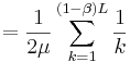
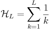
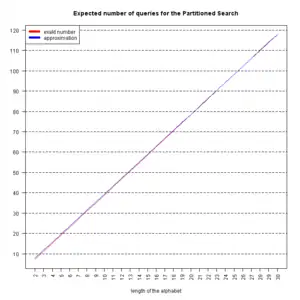 expected number of queries (L=28)  , the expected number of queries. Interestingly, this can be stated as a finite sum , the expected number of queries. Interestingly, this can be stated as a finite sum
If N is big, we have
|
| For the alternate search using purely random queries of the entire phrase, a sequence of L letters is chosen. The result is either a success and matches the target phrase, or does not. If there is no match, a completely new sequence of letters is chosen. To compare partitioned search to purely random queries, we can rewrite (5) as
|
Here, is simply  . Putting in the values . Putting in the values  , ,  , we get , we get   , while partitioned search takes 104.55 queries on average (the approximation via the harmonic number yields 106.03, not too shabby). , while partitioned search takes 104.55 queries on average (the approximation via the harmonic number yields 106.03, not too shabby). |
| For L =28 and N =27 and moderate values of Q,we have p << q corresponding to a large contribution of active information. The active information is due to knowledge of partial solutions of the target phrase. Without this knowledge, the entire phrase is tagged as “wrong” even if it differs from the target by one character. | So, how big is this active information? For p, it was calculated in section III, A as  , and using the same approximation, we get , and using the same approximation, we get  (that's only true-ish for small values of Q and large alphabets...) But what does this mean? How does active information contribute to anything? At the moment, the reasoning seems to be circular: the active information is great (as the probability of a success is great), therefore the active information contributed much. (that's only true-ish for small values of Q and large alphabets...) But what does this mean? How does active information contribute to anything? At the moment, the reasoning seems to be circular: the active information is great (as the probability of a success is great), therefore the active information contributed much. |
The enormous amount of active information provided by partitioned search is transparently evident when the alphabet is binary. Then, independent of L, convergence can always be performed in two steps. From the first query, the correct and incorrect bits are identified. The incorrect bits are then complemented to arrive at the correct solution. Generalizing to an alphabet of N characters, a phrase of arbitrary length L can always be identified in, at most,  queries. The first character is offered, and the matching characters in the phrase are identified and frozen in place. The second character is offered, and the process is repeated. After repeating the procedure times, any phrase characters not yet identified must be the last untested element in the alphabet. queries. The first character is offered, and the matching characters in the phrase are identified and frozen in place. The second character is offered, and the process is repeated. After repeating the procedure times, any phrase characters not yet identified must be the last untested element in the alphabet. |
Wow, the hangman game |
| Partitioned search can be applied at different granularities. We can, for example, apply partitioned search to entire words rather than individual letters. Let there be W words each with L/W characters each. Then, partitioned search probability of success after Q queries is
|
What's that all about? Imagine an alphabet of 32 letters - including {A,B,...,Z,*} and our weasel-phrase. Then the phrase could also be encoded by 28 5-bit words. One 5-bit word is only correct, if all 5 bits are correct. Therefore, we get the same expressions for N=32, L=28, W=28 and N=2, L=140 and W=28. |
Equations (22) and (23) are special cases for  and and  . If . If  , we can make the approximation , we can make the approximation  from which it follows that the active information is from which it follows that the active information is
With reference to (6), the active information is that of W individual searches: one for each word. |
So, for , we get  As stated before: we have L individual searches... As stated before: we have L individual searches... |
 (22)
(22)  .
.
 , where
  is the Lth
  (23)
(23) . (24)
  . (25)
F. Random Mutation
| Original Text | Annotiations |
|---|---|
In random mutation, the active information comes from the following sources.
|
|
| We now offer examples of measuring the active information for these sources of mutation-based search procedures. |
Choosing the Fittest of a Number of Mutated Offspring
| Original Text | Annotiations |
|---|---|
| In evolutionary search, a large number of offspring is often generated, and the more fit offspring are selected for the next generation. When some offspring are correctly announced as more fit than others, external knowledge is being applied to the search, giving rise to active information. As with the child's game of finding a hidden object, we are being told, with respect to the solution, whether we are getting "colder" or "warmer" to the target. | The evaluation of the fitness function introduces external knowledge. |
Consider the special case where a single parent gives rise to  children. The single child with the best fitness is chosen and used as the parent for the next generation. If there is even a small chance of improvement by mutation, the number of children can always be chosen to place the chance of improvement arbitrarily close to one. children. The single child with the best fitness is chosen and used as the parent for the next generation. If there is even a small chance of improvement by mutation, the number of children can always be chosen to place the chance of improvement arbitrarily close to one. |
children? What is wrong with n, k, j? |
To show this, let  be the improvement in fitness. Let the cumulative distribution of be be the improvement in fitness. Let the cumulative distribution of be  . Requiring there be some chance that a single child will have a better fitness is assured by requiring . Requiring there be some chance that a single child will have a better fitness is assured by requiring  or, equivalently, or, equivalently,  . . |
So,  is our fitness function. Why not. The rest is basic math. is our fitness function. Why not. The rest is basic math. |
Generate children, and choose the single fittest. The resulting change of fitness will be  , where , where  is the change in fitness of child is the change in fitness of child  . It follows that . It follows that  so that the probability the fitness increases is so that the probability the fitness increases is
| |
Since  , this probability can be placed arbitrarily close to one by choosing a large enough number of children . If we define success of a single generation as better fitness, the active information of having children as opposed to one is , this probability can be placed arbitrarily close to one by choosing a large enough number of children . If we define success of a single generation as better fitness, the active information of having children as opposed to one is  |
Now, that's quite a surprise: until now, success meant finding the target. For a single step of our search, the average active information was defined. And now, we look at something quite different. And we get a new baseline...
BTW, the minus sign is an obvious error:
|
 (26)
(26)

Optimization by Mutation
| Original Text | Annotiations |
|---|---|
| Optimization by mutation, a type of stochastic search, discards mutations with low fitness and propagates those with high fitness. To illustrate, consider a single-parent version of a simple mutation algorithm analyzed by McKay [32]. | A simple mutation algorithm analyzed by McKay. One would expect that this analysis is done in [32] This is a book with more than 600 pages, which David MacKay thankfully put online. In Chapter III, 19 :Why have Sex? Information Acquisition and Evolution, a mutation algorithm is discussed briefly, but this is explicitly about algorithms with multiple parents, it just doesn't fit a single parent version - MacKay assumes for instance that the fitness of the parents is normally distributed, something you just can't have for a single parent version. So why do Marks and Dembski give MacKay as a reference? On the other hand, algorithms of this kind are studied since the 1970s, this is for instance an so called evolutionary strategy, more precisely, a (1, )ES. |
Assume a binary ( ) alphabet and a phrase of L bits. The ?rst query consists of L randomly selected binary digits.We mutate the parent with a bit-flip probability of ) alphabet and a phrase of L bits. The ?rst query consists of L randomly selected binary digits.We mutate the parent with a bit-flip probability of  and form two children. The fittest child, as measured by the Hamming distance from the target, serves as the next parent, and the process is repeated. Choosing the fittest child is the source of the active information. When and form two children. The fittest child, as measured by the Hamming distance from the target, serves as the next parent, and the process is repeated. Choosing the fittest child is the source of the active information. When  , the search is , the search is
a simple Markov birth process [34] that converges to the target. |
What is a simple Markov birth process according to [34] A. Papoulis, Probability, Random Variables, and Stochastic Processes, 3rd ed. New York: McGraw-Hill, 1991, pp. 537–542. (The page numbers are wrong. Sloppy, isn't it?) On page 647, we read And on the next page:
|
To show this, let  be the number of correct bits on the nth iteration. For an initialization of be the number of correct bits on the nth iteration. For an initialization of  , we show in the Appendix that the expected value of this iteration is , we show in the Appendix that the expected value of this iteration is
where the overbar denotes expectation. Example simulations are shown in Fig. 2. The endogenous information of the search is
|
To show what? That this is a simple birth process? That is absurd, as a look at Fig. 2 shows. It is a birth process - for small , but it is not a simple one. But that is not what the calculations are about: it's an estimation for the average number of generations it takes to complete the search. Using their appendix, I would have estimated this number by
In the end, it doesn't make much of a difference, as BTW, it's not complicated to make a similar approximation for an alphabet of N instead of 2 letters:
|
A reasonable assumption is that half of the initially chosen random bits are correct, and  . Set . Set  . Then, since the number of queries is . Then, since the number of queries is  , the number of queries for a perfect search ( , the number of queries for a perfect search ( ) is ) is
|
 approx. vs. reality for L=100
If we define success of a single generation as better fitness, the active information of having two children as opposed to one is |
For the example shown in Fig. 2, 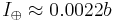 per query. per query. |
Just inserting the parameters of the example in Fig. 2 ( ) into their wrong formula gives you this number. But there is another problem: for the math they made the assumption that half of the initially chosen random bits are correct (), while all the processes in Fig. 2 start with all of the initially chosen random bits being false ( ) into their wrong formula gives you this number. But there is another problem: for the math they made the assumption that half of the initially chosen random bits are correct (), while all the processes in Fig. 2 start with all of the initially chosen random bits being false ( ). ).
|
 consisting of a family of increasing staircase functions. The process
  and increases by 1 at the discontinuity points
  (birth times).
 :
: 
 (28)
(28) bits. Let us estimate that this information is achieved by a perfect search in G generations when
  and
and  is very close to one. Assume
  . Then
 .
.
 . The expected number of queries would be two times of this - as there are two children in each generation:
 .
.
 .
. .
The average active information per query is thus
.
The average active information per query is thus
 or, since
  for
for  .
. .
. . For the example in Fig. 2, Marks and Dembski therefore take
  for
for  .
.
 . But what's about the calculations of the previous paragraph? Remember
  ? Using the appendix, we get for the current problem
  and
and  , so
, so  .
.  . What does this mean?
  and
and  .
. and
and  .
.Optimization by Mutation With Elitism:
| Original Text | Annotiations |
|---|---|
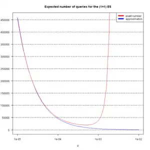
| Optimization by mutation with elitism is the same as optimization by mutation in Section III-F2 with the following change. One mutated child is generated. If the child is better than the parent, it replaces the parent. If not, the child dies, and the parent tries again. Typically, this process gives birth to numerous offspring, but we will focus attention on the case of a single child. We will also assume that there is a single bit flip per generation. | Interesting name: Generally, this well-known algorithm is called (1+1)ES. Though the single bit flip is an amusing twist, usually, the mutation procedure works like the one of the last paragraph, i.e., every bit is flipped with a certain probability . |
For L bits, assume that there are k matches to the target. The chance of improving the fitness is a Bernoulli trial with probability  . The number of Bernoulli trials before a success is geometric random variable equal to the reciprocal . The number of Bernoulli trials before a success is geometric random variable equal to the reciprocal  . We can use this property to map the convergence of optimization by mutation with elitism. For discussion’s sake, assume we start with an estimate that is opposite of the target at every bit. The initial Hamming distance between the parent and the target is thus L. The chance of an improvement on the first flip is one, and the Hamming distance decreases to L - 1. The chance of the second bit flip to improve the fitness is . We can use this property to map the convergence of optimization by mutation with elitism. For discussion’s sake, assume we start with an estimate that is opposite of the target at every bit. The initial Hamming distance between the parent and the target is thus L. The chance of an improvement on the first flip is one, and the Hamming distance decreases to L - 1. The chance of the second bit flip to improve the fitness is  . We expect flips before the next improvements. The sum of the expected values to achieve a fitness of L - 2 is therefore . We expect flips before the next improvements. The sum of the expected values to achieve a fitness of L - 2 is therefore
|
The whole section doesn't bring any new thoughts, just a new labeling:  instead of instead of  . It's just a shortcut for the math done in the appendix. Let's do the math for the usual mutation procedure, i.e., each letter is flipped with probability . Then one would expect . It's just a shortcut for the math done in the appendix. Let's do the math for the usual mutation procedure, i.e., each letter is flipped with probability . Then one would expect  tries to get from k correct letters to (k+1) correct letters. Similar to the calculation above, starting with tries to get from k correct letters to (k+1) correct letters. Similar to the calculation above, starting with  letters in place, we'll need letters in place, we'll need
We can even use an alphabet with N letters, and get
|
| Likewise
or, in general,
It follows that
where
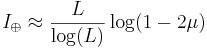
is the Lth harmonic number [3]. Simulations are shown in Fig. 3, and a comparison of their average with (30) is in Fig. 4. For l = L, we have a perfect search and
This is shown in Fig. 5. |
One flipped letter per phrase translates to a mutation rate of  on average. Here we can see that - for small - (1+1)ES takes twice the number of generations as (1,2)ES - though the number of queries the same! on average. Here we can see that - for small - (1+1)ES takes twice the number of generations as (1,2)ES - though the number of queries the same!
2) Optimization by Mutation and 3) Optimization by Mutation With Elitism are hopefully written by different authors - otherwise, the inconsistency of the notation would be embarrassing. And there is no need that the example for section 2) has 100 b, while the example for section 3) has 131 b (why 131?). Or that the algorithm in 2) start with 50 correct bits, while in 3) it starts at zero. Especially hard to understand is that the similarity of
hasn't been spotted. |
| Since the endogenous information is L bits, the active information per query is therefore
|
You get the same result for the (1+1)ES of the last section if you set  : :
|
 .
. ).
). .
.
 (29)
(29) (30),
(30),
 .
. and
and
 bits per query.

 .
.