Williamson's model of managerial discretion

Oliver E. Williamson hypothesised (1964) that profit maximization would not be the objective of the managers of a joint stock organisation.[1] This theory, like other managerial theories of the firm, assumes that utility maximisation is a manager’s sole objective.[2] However it is only in a corporate form of business organisation that a self-interest seeking manager maximise his/her own utility, since there exists a separation of ownership and control.[3] The managers can use their ‘discretion’ to frame and execute policies which would maximise their own utilities rather than maximising the shareholders’ utilities. This is essentially the principal–agent problem.[4] This could however threaten their job security, if a minimum level of profit is not attained by the firm to distribute among the shareholders.[5]

The basic assumptions of the model are:

1. Imperfect competition in the markets.
2. Divorce of ownership and management.
3. A minimum profit constraint exists for the firms to be able to pay dividends to their share holders.[6]

Managerial utility function

The managerial utility function includes variables such as salary, job security, power, status, dominance, prestige and professional excellence of managers. Of these, salary is the only quantitative variable and thus measurable. The other variables are non-pecuniary, which are non-quantifiable. The variables expenditure on staff salary, management slack, discretionary investments can be assigned nominal values. Thus these will be used as proxy variables to measure the real or unquantifiable concepts like job security, power, status, dominance, prestige and professional excellence of managers, appearing in the managerial utility function.[7]

Utility function or "expense preference"[8] of a manager can be given by:

${\displaystyle U=U(S,M,I_{D})\,}$

where U denotes the Utility function, S denotes the “monetary expenditure on the staff”, M stands for "Management Slack" and I_D stands for amount of "Discretionary Investment".

"Monetary expenditure on staff" include not only the manager's salary and other forms of monetary compensation received by him from the business firm but also the number of staff under the control of the manager as there is a close positive relationship between the number of staff and the manager's salary.

"Management slack" consists of those non-essential management perquisites such as entertainment expenses, lavishly furnished offices, luxurious cars, large expense accounts, etc. which are above minimum to retain the managers in the firm. These perks, even if not provided would not make the manager quit his job, but these are incentives which enhance their prestige and status in the organisation in turn contributing to efficiency of the firm's operations. The Management Slack is also a part of the cost of production of the firm.

"Discretionary investment" refers to the amount of resources left at a manager's disposal, to be able to spend at his own discretion. For example, spending on latest equipment, furniture, decoration material, etc. It satisfies their ego and gives them a sense of pride. These give a boost to the manager's esteem and status in the organisation. Such investments are over and above the amount required for the survival of the firm (such as periodic replacement of the capital equipment).[3][7]

Concepts of profit in the model

The various concepts of profit used in the model needs to be understood clearly before moving to the main model. Williamson has put forth four main concepts of profits in his model:

Actual profit (Π)

${\displaystyle \Pi =R-C-S\,}$

where R is the total revenue, C is the cost of production and S is the staff expenditure.

Reported profit (Π_r)

${\displaystyle \Pi _{r}=\Pi -M\,}$

where Π is the actual profit and M is the management slack.

Minimum profit (Π₀)

It is the amount of profit after tax deducted which should be paid to the shareholders of the firm, in the form of dividends, to keep them satisfied. If the minimum level of profit cannot be given out to the shareholders, they might resort of bulk sale of their shares which will transfer the ownership to other hands leaving the company in the risk of a complete take over. Since the shareholders have the voting rights, they might also vote for the change of the top level of management. Thus the job security of the manager is also threatened.[8] Ideally the reported profits must be either equal to or greater than the minimum profits plus the taxes, as it is only after paying out the minimum profit that the additional profit can be used to increase the managerial utility further.

${\displaystyle \Pi _{r}\geq \Pi _{0}+T\,}$

where Π_r is the reported profit, Π₀ is the minimum profit and T is the tax.

Discretionary profit (Π_D)

It is basically the entire amount of profit left after minimum profits and tax which is used to increase the manager’s utility, that is, to pay out managerial emoluments as well as allow them to make discretionary investments.

${\displaystyle \Pi _{D}=\Pi -\Pi _{0}-T\,}$

where Π_D is the discretionary profit, Π is the actual profit, Π₀ is the minimum profit and T is the tax amount.

However, what appears in the managerial utility function is discretionary investments (I_D) and not discretionary profits. Thus it is very important to distinguish between the two as further in the model we would have to maximize the managerial utility function given the profit constraint.

${\displaystyle I_{D}=\Pi _{r}-\Pi _{0}-T\,}$

where Π_r is the reported profit, Π₀ is the minimum profit and T is the tax amount.

Thus it can be seen that the difference in the Discretionary Profit and the Discretionary investment arises because of the amount of managerial slack. This can be represented by the given equation

${\displaystyle \Pi _{D}=I_{D}+M\,}$

where Π_D is the discretionary profit, I_D is the Discretionary investment and M is the management slack.[3][9]

Model framework

For simple representation of the model the managerial slack is considered to be zero. Thus there is no difference between the actual profit and reported profit, which implies that the discretionary profit is equal to the discretionary investment. I.e.

${\displaystyle \Pi _{r}=\Pi {\text{ or }}\Pi _{D}=I_{D}\,}$

where Π_r is the reported profit, Π is the actual profit, Π_D is the discretionary profit and I_D is the discretionary investment.

Such that the utility function of the manager becomes

${\displaystyle U=U(S,I_{D})\,}$

where S is the staff expenditure and I_D is the discretionary investment.

There is a trade off between these two variables. Increase in either will give the manager a higher level of satisfaction. At any point of time the amount of both these variables combined is the same, therefore an increase in one would automatically require a decrease in the other. The manager therefore has to make a choice of the correct combination of these two variables to attain a certain level of desired utility.[3][4]

Substituting

${\displaystyle I_{D}=\Pi -\Pi _{0}-T\,}$ in the new managerial utility function, it can be rewritten as

${\displaystyle U=U(S,\Pi -\Pi _{0}-T)\,}$

The relationship between the two variables in the manager’s utility function is determined by the profit function. Profit of a firm is dependent on the demand and cost conditions. Given the cost conditions the demand is dependent of the price, staff expenditures and the market condition.

${\displaystyle X=f(S,{\bar {P}},{\bar {E}})\,}$

Price and market condition is assumed to be given exogenously at equilibrium. Thus the profit of the firm becomes dependent on the staff expenditure which can be written as

${\displaystyle \Pi =f(X)=f(S,{\bar {P}},{\bar {E}})\,}$

Discretionary profit can be rewritten as

${\displaystyle \Pi _{D}=f(S,{\bar {P}},{\bar {E}})-\Pi _{0}-T)\,}$

In the model, the managers would try to maximise their utility given the profit constraint

${\displaystyle \max U=U(S,\Pi -\Pi _{0}-T)\,}$

${\displaystyle {\text{subject to}}\Pi \geq \Pi _{0}+T\,}$[8]

Graphical representation of the model

Fig 1. Utility indifference curves of managers

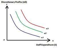
Fig 1. shows the various levels of utility (U₁, U₂, U₃) derived by the manager by combining different amounts of discretionary profits and staff expenditure. Higher the indifference curve, higher is the level of utility derived by the manager. Hence the manager would try to be on the highest level of indifference curve possible given the constraints. Staff expenditure is plotted on the x-axis and discretionary profits on the y-axis.

The discretionary profit in this simplified model is equal to the discretionary investment. The indifference curves are downward sloping and convex to the origin. This shows diminishing marginal rate of substitution of staff expenditure for discretionary profits. The curves are asymptotic in nature which implies that at any point of time and under any given circumstance the manager will choose positive amounts of both discretionary profits and staff expenditure.[8]

Fig 2. Discretionary profit curve

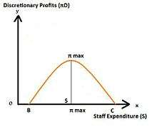
Assuming that the firm is producing an optimum level of output and the market environment is given, the discretionary profits curve is generated, shown in Fig 2. It gives the relationship between staff expenditure and discretionary profits.

It can be seen from the figure that profit will be positive in the region between the points B and C. Initially with increase in profits, the staff expenditure the discretionary profits also increase, but this is only till the point Π_max, that is, till S level of staff expenditure. Beyond this if staff expenditure is increased due to increase in output, then a fall in the discretionary profits is noticed. Staff expenditure of less than B and more than C is not feasible as it wouldn't satisfy the minimum profit constraint and would in turn threaten the job security of managers.[5]

Fig 3. Equilibrium of a firm in Williamson's Model

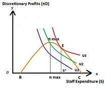
To find the equilibrium in the model, Fig 1. is superimposed on Fig 2. The equilibrium point is the point where the discretionary profit curve is tangent to the highest possible indifference curve of the manager, which is point E in Fig 3. Staying at the highest profit point would require the manager to be at a lower indifference curve U₂. In this case the highest attainable level of utility is U₃. At equilibrium, the level of profits would be lower but staff expenditure S* is higher than the staff expenditure made at the maximum profit point. As indifference curve is downward sloping, the equilibrium point would always be on the right of the maximum profit point. Thus the model shows the higher preference of managers for staff expenditure as compared to the discretionary investments.[3]

Criticism

1. The model fails to describe how businesses take their price and output decisions in a highly competitive set up.[1]
2. The relationship between better performance of managers and the increasing amounts spent on manager’s utility by the firm is not always true.[6]
3. The model does not apply in a dynamic set up like changing demand and cost conditions during booms and recessions.[3]

See also

• Theory of the firm
• Oliver E. Williamson
• Principal–agent problem

References

1. International Management Journal, Kenny Crossan, The Theory of the Firm and Alternative Theories of Firm Behaviour: A Critique. International Journal of Applied Institutional Governance Volume 1 Issue 1; ISSN 1747-6259.
2. D. D. Tewari, Katar Singh (2003). Principles of Microeconomics. New Age International Publishers. pp. 92. ISBN 81-224-1017-0.
3. H.L. Ahuja (2009). Advanced Economic Theory. S.Chand&Co. pp. 932. ISBN 81-219-0260-6.
4. Geetika, Piyali Ghosh, Purba Roy Choudhury (2009). Managerial Economics. The McGraw-Hill Companies. pp. 50. ISBN 978-0-07-026365-9.
5. Mukund Mahajan (2008). Managerial Economics, third edition. Nirali Prakashan. pp. 10.15.
6. Objectives of Firms, SMU WordPress. MB0042-Unit-06.
7. E. Narayanan Nadar, S. Vijayan (2009). Managerial Economics, eastern economy edition. PHI Learning Pvt. Ltd. pp. 42. ISBN 978-81-203-3720-6.
8. M. L. Trivedi (2009). Managerial Economics: Theory and Applications. Tata McGraw–Hill. pp. 100. ISBN 978-0-07-043578-0.
9. Maria Moschandreas (2005). Business Economics, second edition. Thomson. p. 204. ISBN 1-86152-399-8.

External links

• http://www.websukat.com/SMU-Books/Managerial-Economics/6-Objectives-Of-Firms.pdf
• http://etd.fcla.edu/UF/UFE1000145/misangyi_v.pdf
• http://www.irs.princeton.edu/pubs/pdfs/406.pdf