Neighbor joining

In bioinformatics, neighbor joining is a bottom-up (agglomerative) clustering method for the creation of phylogenetic trees, created by Naruya Saitou and Masatoshi Nei in 1987.[1] Usually used for trees based on DNA or protein sequence data, the algorithm requires knowledge of the distance between each pair of taxa (e.g., species or sequences) to form the tree.[2]

The algorithm

Starting with a star tree (A), the Q matrix is calculated and used to choose a pair of nodes for joining, in this case f and g. These are joined to a newly created node, u, as shown in (B). The part of the tree shown as solid lines is now fixed and will not be changed in subsequent joining steps. The distances from node u to the nodes a-e are computed from equation (3). This process is then repeated, using a matrix of just the distances between the nodes, a,b,c,d,e, and u, and a Q matrix derived from it. In this case u and e are joined to the newly created v, as shown in (C). Two more iterations lead first to (D), and then to (E), at which point the algorithm is done, as the tree is fully resolved.

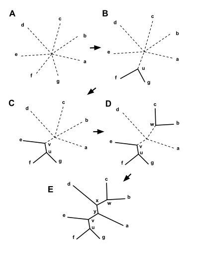
Neighbor joining takes as input a distance matrix specifying the distance between each pair of taxa. The algorithm starts with a completely unresolved tree, whose topology corresponds to that of a star network, and iterates over the following steps until the tree is completely resolved and all branch lengths are known:

1. Based on the current distance matrix calculate the matrix ${\displaystyle Q}$ (defined below).
2. Find the pair of distinct taxa i and j (i.e. with ${\displaystyle i\neq j}$) for which ${\displaystyle Q(i,j)}$ has its lowest value. These taxa are joined to a newly created node, which is connected to the central node. In the figure at right, f and g are joined to the new node u.
3. Calculate the distance from each of the taxa in the pair to this new node.
4. Calculate the distance from each of the taxa outside of this pair to the new node.
5. Start the algorithm again, replacing the pair of joined neighbors with the new node and using the distances calculated in the previous step.

The Q-matrix

Based on a distance matrix relating the ${\displaystyle n}$ taxa, calculate ${\displaystyle Q}$ as follows:

${\displaystyle Q(i,j)=(n-2)d(i,j)-\sum _{k=1}^{n}d(i,k)-\sum _{k=1}^{n}d(j,k)}$

(1)

where ${\displaystyle d(i,j)}$ is the distance between taxa ${\displaystyle i}$ and ${\displaystyle j}$.

Distance from the pair members to the new node

For each of the taxa in the pair being joined, use the following formula to calculate the distance to the new node:

${\displaystyle \delta (f,u)={\frac {1}{2}}d(f,g)+{\frac {1}{2(n-2)}}\left[\sum _{k=1}^{n}d(f,k)-\sum _{k=1}^{n}d(g,k)\right]\quad }$

(2)

and:

${\displaystyle \delta (g,u)=d(f,g)-\delta (f,u)\quad }$

Taxa ${\displaystyle f}$ and ${\displaystyle g}$ are the paired taxa and ${\displaystyle u}$ is the newly created node. The branches joining ${\displaystyle f}$ and ${\displaystyle u}$ and ${\displaystyle g}$ and ${\displaystyle u}$, and their lengths, ${\displaystyle \delta (f,u)}$ and ${\displaystyle \delta (g,u)}$ are part of the tree which is gradually being created; they neither affect nor are affected by later neighbor-joining steps.

Distance of the other taxa from the new node

For each taxon not considered in the previous step, we calculate the distance to the new node as follows:

${\displaystyle d(u,k)={\frac {1}{2}}[d(f,k)+d(g,k)-d(f,g)]}$

(3)

where ${\displaystyle u}$ is the new node, ${\displaystyle k}$ is the node which we want to calculate the distance to and ${\displaystyle f}$ and ${\displaystyle g}$ are the members of the pair just joined.

Complexity

Neighbor joining on a set of ${\displaystyle n}$ taxa requires ${\displaystyle n-3}$ iterations. At each step one has to build and search a ${\displaystyle Q}$ matrix. Initially the ${\displaystyle Q}$ matrix is size ${\displaystyle n\times n}$, then the next step it is ${\displaystyle (n-1)\times (n-1)}$, etc. Implementing this in a straightforward way leads to an algorithm with a time complexity of ${\displaystyle O(n^{3})}$; implementations exist which use heuristics to do much better than this on average .

Example

Neighbor joining with 5 taxa. In this case 2 neighbor joining steps give a tree with fully resolved topology. The branches of the resulting tree are labeled with their lengths.

Let us assume that we have five taxa ${\displaystyle (a,b,c,d,e)}$ and the following distance matrix ${\displaystyle D}$:

	a	b	c	d	e
a	0	5	9	9	8
b	5	0	10	10	9
c	9	10	0	8	7
d	9	10	8	0	3
e	8	9	7	3	0

First step

First joining

We calculate the ${\displaystyle Q_{1}}$ values by equation (1). For example:

${\displaystyle Q_{1}(a,b)=(n-2)d(a,b)-\sum _{k=1}^{5}d(a,k)-\sum _{k=1}^{5}d(b,k)}$

${\displaystyle =(5-2)\times 5-(5+9+9+8)-(5+10+10+9)=15-31-34=-50}$

We obtain the following values for the ${\displaystyle Q_{1}}$ matrix (the diagonal elements of the matrix are not used and are omitted here):

	a	b	c	d	e
a		−50	−38	−34	−34
b	−50		−38	−34	−34
c	−38	−38		−40	−40
d	−34	−34	−40		−48
e	−34	−34	−40	−48

In the example above, ${\displaystyle Q_{1}(a,b)=-50}$. This is the smallest value of ${\displaystyle Q_{1}}$, so we join elements ${\displaystyle a}$ and ${\displaystyle b}$.

First branch length estimation

Let ${\displaystyle u}$ denote the new node. By equation (2), above, the branches joining ${\displaystyle a}$ and ${\displaystyle b}$ to ${\displaystyle u}$ then have lengths:

${\displaystyle \delta (a,u)={\frac {1}{2}}d(a,b)+{\frac {1}{2(5-2)}}\left[\sum _{k=1}^{5}d(a,k)-\sum _{k=1}^{5}d(b,k)\right]\quad ={\frac {5}{2}}+{\frac {31-34}{6}}=2}$

${\displaystyle \delta (b,u)=d(a,b)-\delta (a,u)\quad =5-2=3}$

First distance matrix update

We then proceed to update the initial distance matrix ${\displaystyle D}$ into a new distance matrix ${\displaystyle D_{1}}$ (see below), reduced in size by one row and one column because of the joining of ${\displaystyle a}$ with ${\displaystyle b}$ into their neighbor ${\displaystyle u}$. Using equation (3) above, we compute the distance from ${\displaystyle u}$ to each of the other nodes besides ${\displaystyle a}$ and ${\displaystyle b}$. In this case, we obtain:

${\displaystyle d(u,c)={\frac {1}{2}}[d(a,c)+d(b,c)-d(a,b)]={\frac {9+10-5}{2}}=7}$

${\displaystyle d(u,d)={\frac {1}{2}}[d(a,d)+d(b,d)-d(a,b)]={\frac {9+10-5}{2}}=7}$

${\displaystyle d(u,e)={\frac {1}{2}}[d(a,e)+d(b,e)-d(a,b)]={\frac {8+9-5}{2}}=6}$

The resulting distance matrix ${\displaystyle D_{1}}$ is:

	u	c	d	e
u	0	7	7	6
c	7	0	8	7
d	7	8	0	3
e	6	7	3	0

Bold values in ${\displaystyle D_{1}}$ correspond to the newly calculated distances, whereas italicized values are not affected by the matrix update as they correspond to distances between elements not involved in the first joining of taxa.

Second step

Second joining

The corresponding ${\displaystyle Q_{2}}$ matrix is:

	u	c	d	e
u		−28	−24	−24
c	−28		−24	−24
d	−24	−24		−28
e	−24	−24	−28

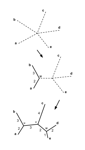
We may choose either to join ${\displaystyle u}$ and ${\displaystyle c}$, or to join ${\displaystyle d}$ and ${\displaystyle e}$; both pairs have the minimal ${\displaystyle Q_{2}}$ value of ${\displaystyle -28}$, and either choice leads to the same result. For concreteness, let us join ${\displaystyle u}$ and ${\displaystyle c}$ and call the new node ${\displaystyle v}$.

Second branch length estimation

The lengths of the branches joining ${\displaystyle u}$ and ${\displaystyle c}$ to ${\displaystyle v}$ can be calculated:

${\displaystyle \delta (u,v)={\frac {1}{2}}d(u,c)+{\frac {1}{2(4-2)}}\left[\sum _{k=1}^{4}d(u,k)-\sum _{k=1}^{4}d(c,k)\right]\quad ={\frac {7}{2}}+{\frac {20-22}{4}}=3}$

${\displaystyle \delta (c,v)=d(u,c)-\delta (u,v)\quad =7-3=4}$

The joining of the elements and the branch length calculation help drawing the neighbor joining tree as shown in the figure.

Second distance matrix update

The updated distance matrix ${\displaystyle D_{2}}$ for the remaining 3 nodes, ${\displaystyle v}$, ${\displaystyle d}$, and ${\displaystyle e}$, is now computed:

${\displaystyle d(v,d)={\frac {1}{2}}[d(u,d)+d(c,d)-d(u,c)]={\frac {7+8-7}{2}}=4}$

${\displaystyle d(v,e)={\frac {1}{2}}[d(u,e)+d(c,e)-d(u,c)]={\frac {6+7-7}{2}}=3}$

	v	d	e
v	0	4	3
d	4	0	3
e	3	3	0

Final step

The tree topology is fully resolved at this point. However, for clarity, we can calculate the ${\displaystyle Q_{3}}$ matrix. For example:

${\displaystyle Q_{3}(v,e)=(3-2)d(v,e)-\sum _{k=1}^{3}d(v,k)-\sum _{k=1}^{3}d(e,k)=3-7-6=-10}$

	v	d	e
v		−10	−10
d	−10		−10
e	−10	−10

For concreteness, let us join ${\displaystyle v}$ and ${\displaystyle d}$ and call the last node ${\displaystyle w}$. The lengths of the three remaining branches can be calculated:

${\displaystyle \delta (v,w)={\frac {1}{2}}d(v,d)+{\frac {1}{2(3-2)}}\left[\sum _{k=1}^{3}d(v,k)-\sum _{k=1}^{3}d(d,k)\right]\quad ={\frac {4}{2}}+{\frac {7-7}{2}}=2}$

${\displaystyle \delta (w,d)=d(v,d)-\delta (v,w)=4-2=2}$

${\displaystyle \delta (w,e)=d(v,e)-\delta (v,w)=3-2=1}$

The neighbor joining tree is now complete, as shown in the figure.

Conclusion: additive distances

This example represents an idealized case: note that if we move from any taxon to any other along the branches of the tree, and sum the lengths of the branches traversed, the result is equal to the distance between those taxa in the input distance matrix. For example, going from ${\displaystyle d}$ to ${\displaystyle b}$ we have ${\displaystyle 2+2+3+3=10}$. A distance matrix whose distances agree in this way with some tree is said to be 'additive', a property which is rare in practice. Nonetheless it is important to note that, given an additive distance matrix as input, neighbor joining is guaranteed to find the tree whose distances between taxa agree with it.

Neighbor joining as minimum evolution

Neighbor joining may be viewed as a greedy heuristic for the Balanced Minimum Evolution[3] (BME) criterion. For each topology, BME defines the tree length (sum of branch lengths) to be a particular weighted sum of the distances in the distance matrix, with the weights depending on the topology. The BME optimal topology is the one which minimizes this tree length. Neighbor joining at each step greedily joins that pair of taxa which will give the greatest decrease in the estimated tree length. This procedure does not guarantee to find the optimum for the BME criterion, although it often does and is usually quite close.

Advantages and disadvantages

The main virtue of NJ is that it is fast[4]^:466 as compared to least squares, maximum parsimony and maximum likelihood methods.[4] This makes it practical for analyzing large data sets (hundreds or thousands of taxa) and for bootstrapping, for which purposes other means of analysis (e.g. maximum parsimony, maximum likelihood) may be computationally prohibitive.

Neighbor joining has the property that if the input distance matrix is correct, then the output tree will be correct. Furthermore, the correctness of the output tree topology is guaranteed as long as the distance matrix is 'nearly additive', specifically if each entry in the distance matrix differs from the true distance by less than half of the shortest branch length in the tree.[5] In practice the distance matrix rarely satisfies this condition, but neighbor joining often constructs the correct tree topology anyway.[6] The correctness of neighbor joining for nearly additive distance matrices implies that it is statistically consistent under many models of evolution; given data of sufficient length, neighbor joining will reconstruct the true tree with high probability. Compared with UPGMA and WPGMA, neighbor joining has the advantage that it does not assume all lineages evolve at the same rate (molecular clock hypothesis).

Nevertheless, neighbor joining has been largely superseded by phylogenetic methods that do not rely on distance measures and offer superior accuracy under most conditions. Neighbor joining has the undesirable feature that it often assigns negative lengths to some of the branches.

Implementations and variants

There are many programs available implementing neighbor joining. RapidNJ and NINJA are fast implementations with typical run times proportional to approximately the square of the number of taxa. BIONJ and Weighbor are variants of neighbor joining which improve on its accuracy by making use of the fact that the shorter distances in the distance matrix are generally better known than the longer distances. FastME is an implementation of the closely related balanced minimum evolution method.

See also

• Nearest neighbor search
• UPGMA and WPGMA
• Minimum Evolution

References

1. Saitou, N.; Nei, M. (1 July 1987). "The neighbor-joining method: a new method for reconstructing phylogenetic trees". Molecular Biology and Evolution. 4 (4): 406–425. doi:10.1093/oxfordjournals.molbev.a040454. PMID 3447015.
2. Xavier Didelot (2010). "Sequence-Based Analysis of Bacterial Population Structures". In D. Ashley Robinson; Daniel Falush; Edward J. Feil (eds.). Bacterial Population Genetics in Infectious Disease. John Wiley and Sons. pp. 46–47. ISBN 978-0-470-42474-2.
3. Gascuel O, Steel M (2006). "Neighbor-joining revealed". Mol Biol Evol. 23 (11): 1997–2000. doi:10.1093/molbev/msl072. PMID 16877499.
4. Kuhner, M. K.; Felsenstein, J. (1994-05-01). "A simulation comparison of phylogeny algorithms under equal and unequal evolutionary rates". Molecular Biology and Evolution. 11 (3): 459–468. doi:10.1093/oxfordjournals.molbev.a040126. ISSN 0737-4038. PMID 8015439.
5. Atteson K (1997). "The performance of neighbor-joining algorithms of phylogeny reconstruction", pp. 101–110. In Jiang, T., and Lee, D., eds., Lecture Notes in Computer Science, 1276, Springer-Verlag, Berlin. COCOON '97.
6. Mihaescu R, Levy D, Pachter L (2009). "Why neighbor-joining works". Algorithmica. 54 (1): 1–24. arXiv:cs/0602041. doi:10.1007/s00453-007-9116-4.CS1 maint: multiple names: authors list (link)

Other sources

• Studier JA, Keppler KJ (1988). "A note on the Neighbor-Joining algorithm of Saitou and Nei". Mol Biol Evol. 5 (6): 729–731. doi:10.1093/oxfordjournals.molbev.a040527. PMID 3221794.
• Martin Simonsen; Thomas Mailund; Christian N. S. Pedersen (2008). Rapid Neighbour Joining (PDF). Proceedings of WABI. Lecture Notes in Computer Science. 5251. pp. 113–122. CiteSeerX 10.1.1.218.2078. doi:10.1007/978-3-540-87361-7_10. ISBN 978-3-540-87360-0.

External links

• The Neighbor-Joining Method — a tutorial