4
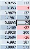
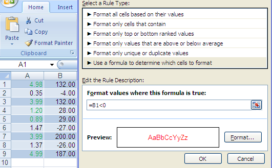
I have an excel worksheet and two columns. I highlight the first column if the value of the cells are less than 0.
Now how can I highlight the second column cells based on the first columns that are highlighted?
See the image below :
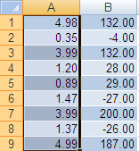
Now I want to make my worksheet like this image:


Pooya Yazdani
Posted 2014-01-01T12:34:44.153
Reputation: 155


How can I apply to whole column, not one by one. You said "Select the range" and in step 3 you said "Put the formula =B1>0". I want to highlight A1 to A10 cells according to B1 to B10, but this formula highlights A1 to A10 according to B1, – Pooya Yazdani – 2014-01-01T13:05:37.557
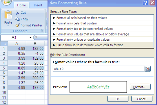
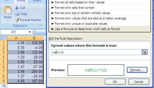
@PooyaYazdani Did you try it? The conditional formatting adapts to the ranges, so that on A2, the actual formula that applies is
=B2>0. – Jerry – 2014-01-01T13:20:26.6931yes I tried it, it doesn't adapt a range to another range! you can simulate this table, I select the first range (A1-A10) an then choose highlight rule, then I select more rules, then Use a formula to determine which cells to format, and then I select second range (B1-B10), but the first range highlights according to first cell of second cell (B1), Is it true? you can simulate this table. – Pooya Yazdani – 2014-01-01T14:53:56.373
@PooyaYazdani I didn't make any mention of selecting the second range! Just put the formula I told in my answer in the box and you'll see! – Jerry – 2014-01-01T15:24:46.030
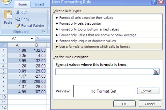
what do you exactly mean by step 2? which option? where should I put the formula? – Pooya Yazdani – 2014-01-01T16:06:38.017
@PooyaYazdani I added pictures. – Jerry – 2014-01-01T16:21:36.147
Great Appreciates Jerry. – Pooya Yazdani – 2014-01-01T16:44:04.677