Linking dropdown lists

Question

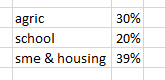
I would want to link a drop-down list to the values of an adjacent cell. Let say, we have two cells A2 and B2. A2 is a drop-down list with values: Agric, school, sme and housing, while B2, which is also a dropdown list, contains percentages: 30%,20% and 39%, respectively for agric, school and sme & housing such that when I select agric from the dropdown list in A2, B2 to displays 30% in that order. how do I go about that?

Answer 1

Lookup tables were designed for this exact purpose. I would use a drop down list in A2 and a VLOOKUP to a table in B2, since it only makes sense to have one drop-down list. If you want the values of B to be tied to the values of A, it makes sense that you're only going to be selecting the value of A, not both A and B. I would do this:

• In some range of cells, either in a separate, protected sheet or elsewhere in the current sheet, create a lookup table like this. In this example, the table is arbitrarily located in cells H7:I9.

• Highlight the column of the lookup table that contains the categories (agric, school, etc.) and created a named ranged for these categories by clicking Formulas, Name Manager, New. The named range should automatically fill in the "Refers To" field with these cells.

• In cell A2, create the drop-down list by clicking Data, Data Validation. Under Allow, specify List, and in the Source field, enter = and the name of your named range. In the screenshot, I used "categories."

• In cell B2, use VLOOKUP to look up the value of A2, which is restricted to the categories in the lookup table, in the columns of the table. This formula works: =VLOOKUP(A2, $H$7:$I$9, 2, FALSE). The 2 indicates that you want the value in the second column of the table, from the row whose first element matches the lookup value (A2). The boolean argument FALSE tells Excel to perform an exact match. If you enter data in column A that doesn't exist in the table, Excel will return #N/A. If you don't enter FALSE, Excel will simply return the last item in the table.

Now, the values in A2 are restricted to the categories in the lookup table, and the value in B2 should automatically update according to the respective percentage for that category. If you want to add new categories, simply add them to the lookup table in the same fashion and update the named range.