2
Picture column A full of comments like feedback from a survey question. Now picture column B with a formula which counts occurrances of particular key words within each comment. I am currently using this formula in column B: SUM(COUNTIF(A27,{"LBNL","Lawrence Berkeley","LBL","Lawrence Lab*"}))
Since the list will be growing and shrinking along the way and because I am going to end up with multiple similar formulas (for different categories) I would like to instead control the list in a named range and reference it from there.
So now let's say my list is like below and has name range of search_items1
- LBNL
- Lawrence Berkeley
- LBL
- Lawrence Lab
My formula would then look like SUM(COUNTIF(A27,search_items1)).
Notice the use of * for wildcard which introduces another challenge but I can't get the above formula to work even without the *. Is there a way to make this work? The solution with the wildcard * would be ideal.
Alternatively could I reference one cell that is concatenated together from the name range and would look like this: {"LBNL","Lawrence Berkeley","LBL","Lawrence Lab*"}. I attempted this but the formula interprets it as one text block.
I have tried multiple syntax variations and countless Google and Super User searches. Please help.

daniellopez46
Posted 2013-09-09T17:58:21.940
Reputation: 233


btw I am trying to avoid VBA if at all possible – daniellopez46 – 2013-09-09T17:58:46.380
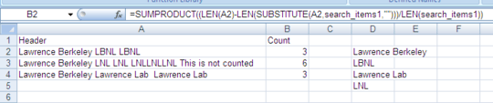
It seems to be working for me and I'm on Excel 2007. The only issue with the current formula is that you're counting in cell A27 only. Also, make sure to use Ctrl+Shift+Enter since the formula is an array function (or use
SUMPRODUCTinstead ofSUM). The namedrange can contain the asterisk and will be considered as wildcard. – Jerry – 2013-09-09T18:04:18.400will what I'm trying to do is for each cell (thus the single cell reference instead of a range) count number of instances for example cell A1 might have "LBNL" or "LBL" or both. In the case of the first two the formula should return 1 and in the case of the second 2. For me it only works for the first item in the name range. So it will count a cell with single text of "LBNL" but if it has "LBNL LBL" it will return 0 instead of 2. Are you sure its working for you? Does it return 2 for you in the latter example? – daniellopez46 – 2013-09-09T18:16:44.840
BTW I tried CSE and using sumproduct and using a range instead but still didn't work: {=SUMPRODUCT(COUNTIF(A27:A27,search_items1))} – daniellopez46 – 2013-09-09T18:18:41.927
1Okay, what you are describing now is not what I had in mind after reading your question. I thought that the column had many comments, and you want to count the number of cells having
LBNL(and nothing else in the same cell), havingLawrence Berkeley, etc and for the 4th text, any cell beginning withLawrence Lab. What you describe now changes everything since you now must put the wildcards to get the result you expect. Put asterisks before and after the text to be counted. And you don't need to use CSE withSUMPRODUCT, that's why I suggested it overSUMwhich you do need. – Jerry – 2013-09-09T18:26:36.567