1
Current Setup
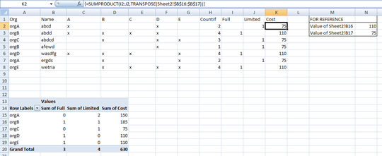
- A table (Table1) that has the following fields:
- Organization Name
- Person Name
- Several fields that users can put an "X" into (each represents a "module" that users would need access to)
- A sum of the # of modules needed (countif on the range for "X" values)
- "full licenses": displays 1 if more than 3 modules needed
- "Limited licenses": display 1 if <= 3 modules needed
- On a separate sheet, two input fields for cost per each full & limited license
Goal
- Create a table showing, per organization, what its cost will be for full and limited license that each Org has selected.
So far
I have been able to create the pivot table showing the number of full and express licenses per organization.
Question
How can I add an additional column to the pivot table that will take the sum for a group (e.g. the sum of # of full licenses for an organization) and multiply that by the cost of the given license type, so that I can calculate the amount each group would owe?

I am confused on what you want to multiply by. Is it B16 and B17 or B22 and B23, per license? – Raystafarian – 2013-07-25T16:58:07.297
The pivot table shows the sum of each type of license per group. I'd essentially like the following additional fields: full license cost (pivot sum * B16), full license maintenance (PT sum * B19), limited license cost (pt sum * B17), and limited license maintenance (pt sum * B20) – SeanKilleen – 2013-07-25T17:15:34.253
Eventually, I'd like to also to sum up the total purchase cost and total yearly cost from the calculated fields I mention in the comment above as well. – SeanKilleen – 2013-07-25T17:16:09.067