Excel Conditional Formatting Multiple Data Bars and Data Icons in one cell

4

5

I am using Excel 2007 on a Windows machine.

I am attempting to place one data bar and one data icon into a cell under the conditional formatting. The issue is that I don't really want to have data icons or data bars for cells that have dates in the future and I only want to have data icons for dates in the at least one month in the past.

This is what I have:
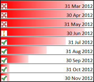
Excel 2007 Databar issue

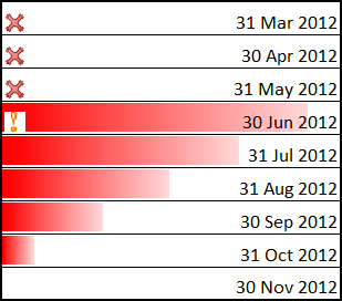
This is what I want:

What I want

I am using the EOMONTH function to determine the last day of the month for the conditional formatting calculations. For the data bar the formula is =EOMONTH(Now(), 4) and =EOMONTH(Now(), -1). The data icons formulas are =EOMONTH(Now(), -1) and =EOMONTH(Now(), -2).

Is there a way in Excel 2007 to get rid of the data icons for all the dates in the future and lose the data bars when the date has past?
wbeard52

Posted 2012-07-07T02:26:46.793

Reputation: 3 149

I haven't had time to play with this, but I can point you in what I think is the right direction. I think you will have to have two or three extra rules and then find the appropriate order and "Stop If True" combination to make this work. – Excellll – 2012-07-07T16:35:56.660

I've played with the Stop if True but they are grayed out for data bars and data icons :-(. The other issue is I can't create a rule to allow one rule to pass while blocking the other rule. – wbeard52 – 2012-07-07T19:35:44.170

I can't even get the data bars to look like your "what I have" pic. Using the two data bar formulas you list above, with the one ending "4" for the minimum, I get increasing bars starting with this month, and none in the past. This makes sense as I'd expect the bars to grow as the formula results, i.e., the dates, get bigger. If I switch the min and max formulas the results don't change. Excel 2010. – Doug Glancy – 2012-07-07T20:23:00.117

The minimum value for the data bar is =EOMONTH(Now(), 4) and the maximum value is =EOMONTH(Now(), -1). If you are using Excel 2010, you need to go to the negative value and axis button and click the very last option box for axis settings - none. – wbeard52 – 2012-07-07T20:39:47.977

Got it. I'd looked at that but not grasped that it applied. – Doug Glancy – 2012-07-07T20:56:04.287

Answers

3

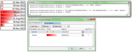
Well, after many hours searching the internet I was able to find an Office Excel Blog that had my answer. http://blogs.office.com/b/microsoft-excel/archive/2006/02/24/conditional-formatting-trick-1-multi-coloured-data-bars.aspx

The idea is to provide a formula for each conditional format to tell it which cells to format and which cells not to format. There is no interface for this built-in to excel so we need to turn to VBA to apply the formulas.

selection.FormatConditions(1).formula = "enter formula here"  
    -- Quotes are mandatory and the Conditional Formats start with "1"
       at the top of the list   
    -- If you make a mistake selection.FormatConditions(1).formula = "=TRUE"

Adding formulas to excel conditional formats

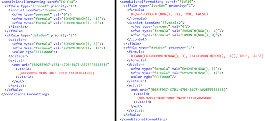
I wasn't sure if this format will persist from one session to the next. I decided to open the Excel file and take a look at its XML contents. In the worksheets folder (after you add the .zip extension to the file), click on the spreadsheet "Sheet1" and at the bottom is the information for the conditional formats. The XML on the left is from before I applied the conditional formats formula and the XML on the right is after.

enter image description here

wbeard52

Posted 2012-07-07T02:26:46.793

Reputation: 3 149

The reference to F6 in the formula comes from the first cell that has the conditional format in the applies to box – wbeard52 – 2015-04-09T17:55:32.960

very interesting! – Doug Glancy – 2012-07-09T15:35:23.457

2

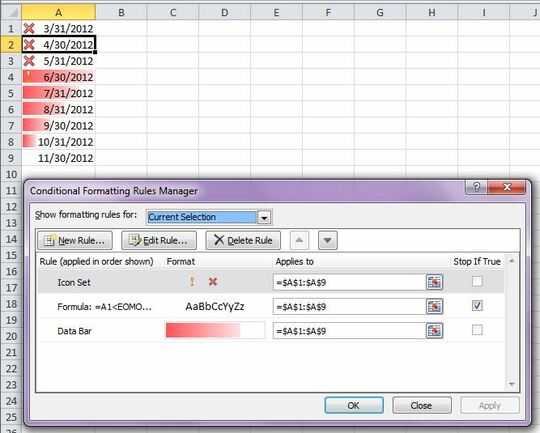
@Excellll hit it on the head a while ago. I spent a while trying different things, but the answer is to add a condition in the middle that makes fills the cell with white if it less than EOMONTH(Now(), -1). Put it in the 2nd position as shown with Stop if True checked. Finally, replace the green checkmark with "No Icon."

enter image description here

EDIT: for Excel 2007

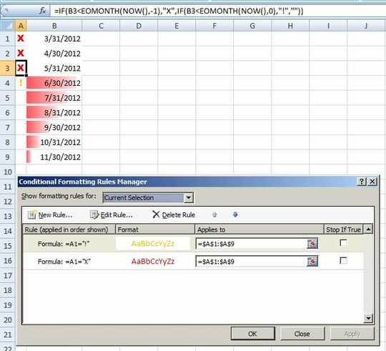
The only way I can think of in XL 2007 is with a helper column. I inserted a column A with this formula:

=IF(B3<EOMONTH(NOW(),-1),"X",IF(B3<EOMONTH(NOW(),0),"!",""))

Then conditionally formatted column A for red font if the cell equals "X" and orange if it equals "!".

You could fiddle with the background color and borders in both sets of cells to make the red flow across. I think. That's my best shot!

enter image description here

Doug Glancy

Posted 2012-07-07T02:26:46.793

Reputation: 1 756

1Doug. How did you get Excel 2007 to show only the two data icons? I know Excel 2010 can do that but I can't seem to figure out how to do that in 2007? – wbeard52 – 2012-07-07T22:08:26.240

I didn't. Sorry, I didn't realize this difference between the two versions. I can't see any way to do it. – Doug Glancy – 2012-07-07T22:55:47.640

Thanks for trying Doug. There has to be a solution though. – wbeard52 – 2012-07-07T23:28:57.747