Change cell color based on other cell value

Question

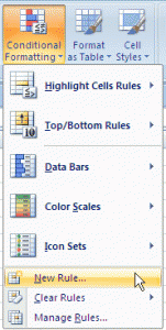
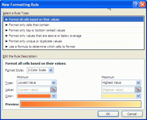
I have encountered numerous questions related to changing a cell color based on its value, which can be achieve easily with Excel "Conditional Formatting". However I'm interested in changing a cell color based on some other cell value.

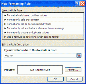
For example, I want cell A4 to be painted red only if cell B4 has a greater value than A4 cell. Is there any way to accomplish that?

I've found this guide which actually explains what I need pretty well, but how can I expand this formatting to numerous cells? Just dragging doesn't work here for me.

EDIT: I'm using the Excel 2007 version.

Answer 1

Conditional formatting in Excel 2007 (based on value of another cell)

1. Select the cell you want to format, “A1″ in this example.
2. In the Home tab, Styles group, click on Conditional Formatting.

3. Select New Rule.

   

4. The New Formatting Rule window will open.

   

5. Click Use a formula to determine which cells to format.

6. The New Formatting Rule window will now look like this:

   

7. In the edit box labeled “Format values where this formula is true“, enter “=” followed by a formula referencing the other cell. In this example the formula: “=B1<0″ is entered.

8. Click the Format button. The Format Cells window will open.

   

9. Specify the formatting you want. In this example I changed the cell color to “RED”.

10. Click OK to close The Format Cells window.

11. Click OK to close The New Formatting Rule window.

To summarize this example: cell A1 will have a RED color when cell B1 value is less than zero.