How to combine values from multiple rows into a single row in Excel?

10

8

I have a data dump in Excel that consists of annual customer data for two different values. The data was provided with a separate row for value for every year and customer. I.e. it looks like this:

enter image description here

I'm stuck with a row for Customer 1 for Value A in 2009 and a separate row for Value B for the same customer in the same year.

In some instances there is no Value A or Value B. In the example above, you can see that Customer 1 has no Value B in 2011, so no row was generated for that. And, though not represented in the example, some clients will have no data for either value in a year (and thus no row for that customer in that year). In that situation, lacking a row for that customer in that year is fine.

I want to get this into a worksheet where there's one row for both values for every year and customer. I.e., I want the data to look like this:

enter image description here

What is the most effective way to create that result?

Greg R.

Posted 2012-02-28T22:05:49.887

Reputation: 1 404

Answers

6

This is VBA, or a macro you can run on your sheet. You must hit alt+F11 to bring up the Visual Basic for Application prompt, go to your workbook and right click - insert - module and paste this code in there. You can then run the module from within VBA by pressing F5. This macro is named "test"

Sub test()
'define variables
Dim RowNum as long, LastRow As long
'turn off screen updating
Application.ScreenUpdating = False
'start below titles and make full selection of data
RowNum = 2
LastRow = Cells.SpecialCells(xlCellTypeLastCell).Row
Range("A2", Cells(LastRow, 4)).Select
'For loop for all rows in selection with cells
For Each Row In Selection
    With Cells
    'if customer name matches
    If Cells(RowNum, 1) = Cells(RowNum + 1, 1) Then
        'and if customer year matches
        If Cells(RowNum, 4) = Cells(RowNum + 1, 4) Then
            'move attribute 2 up next to attribute 1 and delete empty line
            Cells(RowNum + 1, 3).Copy Destination:=Cells(RowNum, 3)
            Rows(RowNum + 1).EntireRow.Delete
        End If
     End If
    End With
'increase rownum for next test
RowNum = RowNum + 1
Next Row
'turn on screen updating
Application.ScreenUpdating = True

End Sub

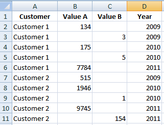
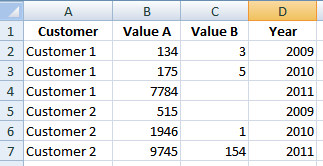
This will run through a sorted spreadsheet and combine consecutive rows that match both the customer and the year and delete the now empty row. The spreadsheet must be sorted the way you've presented it, customers and years ascending, this particular macro won't look beyond consecutive rows.

Edit - it's entirely possible my with statement is completely unneeded, but it's not hurting anyone..

REVISITED 02/28/14

Someone used this answer in another question and when I went back I thought this VBA poor. I've redone it -

Sub CombineRowsRevisited()

Dim c As Range
Dim i As Integer

For Each c In Range("A2", Cells(Cells.SpecialCells(xlCellTypeLastCell).Row, 1))
If c = c.Offset(1) And c.Offset(,4) = c.Offset(1,4) Then
            c.Offset(,3) = c.Offset(1,3)
            c.Offset(1).EntireRow.Delete
End If

Next

End Sub

Revisited 05/04/16

Asked again How to combine values from multiple rows into a single row? Have a module, but need the variables explaining and again, it's pretty poor.

Sub CombineRowsRevisitedAgain()
    Dim myCell As Range
    Dim lastRow As Long
    lastRow = Cells(Rows.Count, "A").End(xlUp).Row

    For Each myCell In Range(Cells("A2"), Cells(lastRow, 1))
        If (myCell = myCell.Offset(1)) And (myCell.Offset(0, 4) = myCell.Offset(1, 4)) Then
            myCell.Offset(0, 3) = myCell.Offset(1, 3)
            myCell.Offset(1).EntireRow.Delete
        End If
    Next
End Sub

However, depending on the problem, it might be better to step -1 on a row number so nothing gets skipped.

Sub CombineRowsRevisitedStep()
    Dim currentRow As Long
    Dim lastRow As Long
    lastRow = Cells(Rows.Count, 1).End(xlUp).Row

    For currentRow = lastRow To 2 Step -1
        If Cells(currentRow, 1) = Cells(currentRow - 1, 1) And _
        Cells(currentRow, 4) = Cells(currentRow - 1, 4) Then
            Cells(currentRow - 1, 3) = Cells(currentRow, 3)
            Rows(currentRow).EntireRow.Delete
        End If
    Next

End Sub

Raystafarian

Posted 2012-02-28T22:05:49.887

Reputation: 20 384

2

Another option:

  1. Select Column B, press CTRL+G -> Special-> Blanks -> OK
  2. Type = press , then CTRL+ENTER
  3. Select Column C, press CTRL+G -> Special-> Blanks -> OK
  4. Type =IF( press type = press press type , press type ,0) then CTRL+ENTER
  5. Select all data and Copy and Paste Special as Values
  6. Remove duplicates.

EDIT:

Explanation: I am trying to make use of GoTo Blanks option. Once you have selected blanks then you can enter the same formula for all selected blank cells. Regarding OP's question, the data looks like have consistent blanks, i.e.: Value A column blanks have the same CustomerID as above nonblank row. In the same way Value B column blanks have the same CustomerID as below nonblank row.

zx8754

Posted 2012-02-28T22:05:49.887

Reputation: 451

Hello zx8754. Could you please add some explanations what the idea behind your solution is? – nixda – 2013-07-17T18:49:31.047

@nixda Explanation added, sorry thought the steps were clear enough. – zx8754 – 2013-07-17T20:56:21.880

0

Everyone is using a lot of VBA code or complicated functions for this. I have a method which takes a second to implement but is far more understandable and very easy to adjust depending on various other possibilities.

In the example you've given above, paste these (4) functions into the cells, E2, F2, G2 and H2, respectively (the F&G functions reference cells above):

=IF(D2=D3, A2,         IF(D2<>D1, A2,            ""))    
=IF(D2=D3, MAX(B2:B3), IF(D2<>D1, B2,            ""))    
=IF(D2=D3, MAX(B2:B3), IF(D2<>D1, IF(C2=0,"",C2),""))    
=IF(D2=D3, D2,         IF(D2<>D1, D2,            ""))

Drag these formulae as far down as necessary. It generates a single row of data each time 2 rows are present, leaving single rows unaffected. Paste special the values (to remove the formulas) of columns E-F-G-H elsewhere and sort them by customer to remove all the extra rows.

Kindlin

Posted 2012-02-28T22:05:49.887

Reputation: 1

0

The most effective way to do this is to dump all of the data into a Pivot Table and drop 'Customer' into Row Labels and then follow up with the other columns. You can drop the 'Year' into the column header if you want to see the breakdown by year

Pivot Tables can be found under Insert in Excel 2010

xXPhenom22Xx

Posted 2012-02-28T22:05:49.887

Reputation: 517

You will run into issues though with cells that have no value in column B because Excel will have no way of knowing that the value in B2 and B3 are in someway related. – xXPhenom22Xx – 2012-02-28T22:22:22.677

I admittedly have little experience with Pivot Tables, but I don't think that Pivot Tables solve the problem I have. I want the data for all the values for a customer in one row per year so I can manipulate it (e.g. create a column adding Value A + Value B), not just change how I'm viewing it via a Pivot Table. I literally want the data structured differently in the worksheet. – Greg R. – 2012-02-28T22:45:25.423

Yea would be tough unless you always had alternating columns with missing data like you do in the example. If this isnt the case then there isnt a way for Excel to logically do what you want it too. – xXPhenom22Xx – 2012-02-28T22:50:40.893

Greg - you can solve the problem thus: once it is in the pivot table in the format you want, copy it out of the pivot table to another location (same sheet or another one) - and then you can manipulate it any way you like, including adding columns, formulas, etc. – yosh m – 2012-02-28T23:19:11.730

0

Here are steps for creating a separate table with the condensed data.

  1. Copy your entire table and paste it on a new sheet.
  2. Select your new table and Remove Duplicates (Data ribbon -> Remove Duplicates) on columns Customer and Year. This will provide the framework for the condensed table.
  3. In B2 (the first entry for Value A) enter the following:

    =IFERROR(INDEX(Sheet1!B$1:B$11,MIN(IF(Sheet1!$A$1:$A$11=$A2,IF(Sheet1!$D$1:$D$11=$D2,IF(Sheet1!B$1:B$11<>"",ROW(Sheet1!$A$1:$A$11),1000000),1000000),1000000))),"")

    Enter the formula as an array formula by pressing Ctrl+Shift+Enter.

  4. Fill the formula down the column. Then fill over to fill the Value B column as well. Voila!

A few notes:

  • You'll of course need to adjust the addresses to fit your data. For reference, Sheet1 is the original data in columns A through D.
  • I'm assuming your data (or headers) starts at Row 1. This is probably true if this is a data dump. The formula will have to be adjusted if this is not the case.
  • I'm assuming your table has fewer than a million rows. If you somehow have more than that, change the 1000000s in the formula to something greater than your number of rows.
  • If your table has many thousand rows (100,000+), you may want to consider using a VBA solution instead since array formulas can get bogged down with large arrays.

Excellll

Posted 2012-02-28T22:05:49.887

Reputation: 11 857