Find missing entries from a list of sequential numbers in a column?

Question

I have an Excel sheet containing the results of 66000 test cases. Or, at least it should...

Now, because I was running the tests asynchronously and kept stopping and starting I had the foresight to make sure the test numbers were put in the output. Now, having used Excel 2007's Remove Duplicates feature based on those test numbers I find I have 65997 rows of data. So three of them are missing.

The job here is to locate the missing task numbers.

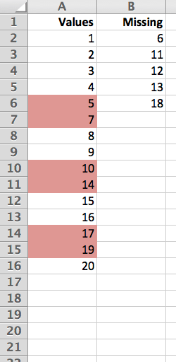
The test numbers are in column A, in ascending order, and there are guaranteed to be no duplicates. Other data is placed in other columns, and these must remain with their test number.

  |    A
--+---------
1 | testNum
2 | 1
3 | 2
4 | 3
5 | ...

Assume there are too many test cases to do this search manually, as I have another data set of closer to a million items that I'm going to have to do a similar job on soon.

I could solve this with VBA, but wonder if there's a more straightforward solution that I'm missing?

Answer 1

Assuming your data is in Column A and begins on row 2, select a range in a free column starting on row 2 and including at least as many rows as you should have results (this is important: if your range includes less cells than your total sequence, the listing of missing results will be truncated)¹. In the formula bar – not directly in the cells! – insert the following formula:

=IFERROR(
   SMALL(
     IF(
       ISNA(MATCH(ROW(A1:A66000)-1,A2:A66001,0)),
       ROW(A1:A66000)-1,
     ""),
   ROW()-1),
 "")

– note this needs to be written on one line; the indentation is just for the sake of readability here. Store it as an array formula by pressing Ctrl+Shift+Enter. If you did this correctly, the formula will display enclosed in braces and Excel will complain when you try to edit single cells in the array range.

For the values in column A of the screenshot below, the formula stored as an array formula in B2:B21 (20 rows because the complete sequence would be 1 to 20) will return the following values in column B:

As you can see, these are the numbers missing in the sequence (highlighted in the screenshot).

---

1. you can err on the generous side when selecting the range to apply as long as the ROW(A1:AXXXXX) reference includes exactly a number of rows equal to your total sequence (66000 rows in your example, hence A1:A66000).

Answer 2

In an empty column (lets assume Z) starting at row 2 put a formula, and copy down for all used rows

=A2=A1+1

Search in column Z for FALSE. will find the test on the row after the missing number

Also you can try

=IF(A2=A1+1,"",A1+1)

Answer 3

This solution requires two helper columns. In Column B, fill down consecutive numbers from 1 to 66,000. In C2 (in the first row of data), enter

=IF(A2=B2,0,1)

In C3, enter

=IF(B3=OFFSET(A3,-1*SUM(C$2:C2),0),0,1)

Fill down C3 to C66001.

From here you can filter B:C to for records with a value of 1 in Column C. This will show the missing numbers.

OR

If you want to get fancy on the last step, you can use this array formula and fill down as far as you require:

=IFERROR(SMALL(IF($C$2:C$32<>0,$B$2:$B$32),ROW()-1),"")

Enter the formula with Ctrl+Shift+Enter. This example was entered in Row 2. You will need to adjust the ROW()-1 in the formula such that this is equal to 1 for the first entry. For example, if you start your list of missing numbers at E5, you'll need to change it to ROW()-4. [Thanks to @kopischke for this method: link]