Excel 2007 Function, last three items

Question

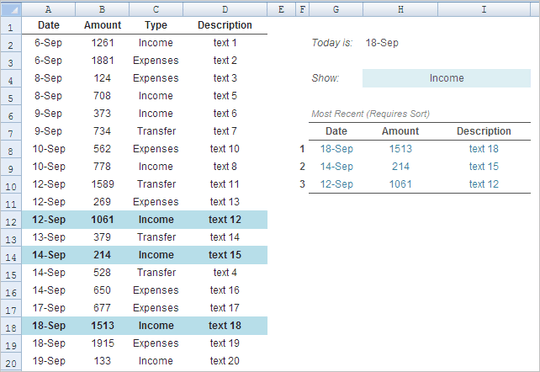
My question is twofold, so bear with the wall of text. I'm making sort of a banking spreadsheet. I will input income/expenses in four columns (Date/Amount/Type/Description) and I need it to keep track of my day to day spending. I already have it so that if the date is not today, it won't add/subtract it until it is. Also, I have it so two/three/four weeks in the future. However, I want to add something to the effect of "Last three paychecks". The "Type" column has only three possible entries, "Income", "Transfer", and "Expense". If I can find a function to work for one, I'm sure I can get it to work with the rest easily. I need it to show the most recent "income" amount. For instance:

Date Amount Type

Sep 1 100 Income

Sep 2 100 Expense

Sep 3 100 Income

Sep 4 100 Expense

Sep 5 100 Income

Sep 6 100 Income

Sep 7 100 Income

Let's say it's Sep 6th today. I would want it to show Sep 5ths amount, Sep 5ths, and Sep 3rds. I don't want it to show expenses, and it's not yet Sep 7th. It would have to be three functions (one for each box), so how would I get it to do the most recent, second to most recent, and so on? If I can get it to work, I can edit to get the description as well, and refit it to expenses if need be.

Question 2:

I would like an "annual checkup" kind of thing. How would I get it to lookup each of every type (same as above), but then have cutoff dates so it's only one year?

Answer 1

This might help you get the three most recent transactions per type. It helps if you've used named ranges for your data sheet.

To get the 3 most recent Income dates, you can use this array formula:

=INDEX(dates,LARGE(ROW(dates)*(dates<=TODAY())*(types="Income"),XXX)-1,1)

Where:

dates -- the cell range/column range that contains the dates
types -- the cell range/column that contains either "Income", "Transfer" or "Expenses"
XXX -- contains either 1 (most recent), 2 (2nd most recent) or 3.

To get the most recent amount and description, replace the first instance of dates in the formula above with the cell range that contains the money amounts and descriptions.

=INDEX(amounts,LARGE(ROW(dates)*(dates<=TODAY())*(types="Income"),XXX)-1,1)

&

=INDEX(descriptions,LARGE(ROW(dates)*(dates<=TODAY())*(types="Income"),XXX)-1,1)

In the example below, dates refers to A2:A100, amounts refers to B2:B100, types refers to C2:C100 and descriptions refers to D2:D100.

In order for the formulas to work, the data table needs to be sorted according to date (oldest to latest). Be sure to commit the formulas using Ctrl + Shift + Enter. This also assumes that there are unique dates for each type of transaction (i.e. no multiple Income entries for a single date).

---

If you don't want to have to sort the table by date, here's an array formula you can try:

=INDEX(dates,
 MATCH(SMALL(IF((dates<=TODAY())*(types="Income"),(TODAY()-dates),""),XXX),
             IF((dates<=TODAY())*(types="Income"),(TODAY()-dates),""),0),1)

Where:

dates -- the cell range/column range that contains the dates
types -- the cell range/column that contains either "Income", "Transfer" or "Expenses"
XXX -- contains either 1 (most recent), 2 (2nd most recent) or 3

Again, to get the most recent amounts and descriptions, replace the first instance of dates in the formula above with the cell range that contains the money amounts and descriptions. Something like this:

=INDEX(amounts,
 MATCH(SMALL(IF((dates<=TODAY())*(types="Income"),(TODAY()-dates),""),XXX),
             IF((dates<=TODAY())*(types="Income"),(TODAY()-dates),""),0),1)

and

=INDEX(descriptions,
 MATCH(SMALL(IF((dates<=TODAY())*(types="Income"),(TODAY()-dates),""),XXX),
             IF((dates<=TODAY())*(types="Income"),(TODAY()-dates),""),0),1)