How do I line up two sets of data in Excel?

If I've got two sets of data, how can I line them up in Excel 2007?

For example, if one set of data has

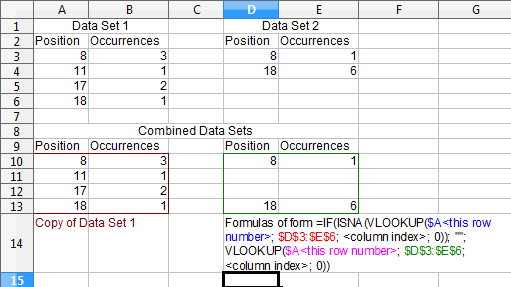
Position    Occurrences
      8               3
     11               1
     17               2
     18               1

and another set of data has

Position    Occurrences
      8               1
     18               6

how can I line it up so that it's

Position    Occurrences     Position    Occurrences
      8               3            8              1
     11               1         
     17               2         
     18               1           18              6

rather than

Position    Occurrences     Position    Occurrences
      8               3            8              1
     11               1           18              6
     17               2         
     18               1

Andrew Grimm

Posted 2011-07-07T01:34:03.440

Reputation: 2 230

I'm struggling trying to figure out a slightly harder example - http://superuser.com/questions/904377/lining-up-sets-of-data-in-excel-with-different-keys. Any ideas?

– Marcus Leon – 2015-04-21T19:47:00.793

I've seen this done, but not done it. If the second list is in a new sheet and sorted on the key (looks like Position), I think you can do an indexed reference. Again, I don't know how, just some hopefully useful details. – Slartibartfast – 2011-07-07T01:44:56.443

2Am I guessing right that the second set could also have data that is not found in the first? Like a row 12 4 and/or a row 20 3? And are the sets always ordered? – Arjan – 2011-07-07T18:19:16.667

Answers

OpenOffice version, which should be easily adapted to Excel (I think the only difference is that OO uses semicolons to separate function arguments, and Excel uses commas):

Given two blocks of data labeled "Data Set 1" (shown below in cells A3:B6) and "Data Set 2" (shown below in cells D3:E6):

Copy Data Set 1 to a new range (shown below in cells A10:B13).
To the right of Data Set 1 (shown in cell D10), enter the following formula:
```
=IF(ISNA(VLOOKUP($A10;$D$3:$E$6;1;0));"";VLOOKUP($A10;$D$3:$E$6;1;0))
```

Adjacent to this cell (shown in cell E10, enter the following formula:

=IF(ISNA(VLOOKUP($A10;$D$3:$E$6;2;0));"";VLOOKUP($A10;$D$3:$E$6;2;0))

Copy and paste cells D10:E10 to cells D11:E13.

The idea behind this is to use VLOOKUP to find cells that match the values in column A. If a matching cell is not found (i.e., the VLOOKUP function returns an N/A value), put an empty string into the cell contents. If a matching cell is found, put the VLOOKUP result into the cell contents.

enter image description here

Mike Renfro

Posted 2011-07-07T01:34:03.440

Reputation: 1 242

This is how I did it under Excel, based on Mike Renfro's answer:

Given two blocks of data labeled "Data Set 1" (shown below in cells A3:B6) and "Data Set 2" (shown below in cells D3:E6):

Copy Data Set 1 to a new range (shown below in cells A10:B13).
To the right of Data Set 1 (shown in cell D10), enter the following formula:
```
=IFERROR(VLOOKUP($A10,$D$3:$E$6,COLUMN()-COLUMN($D10)+1,0),"")
```
Copy and paste this formula to D10:E13

Differences from Mike's answer:

Rather than manually entering the column number, I used the COLUMN formula.
Rather than doing VLOOKUP twice, I did it once, and then used IFERROR if it can't find anything.
I used commas rather than semicolons, as Mike noted.

Andrew Grimm

Posted 2011-07-07T01:34:03.440

Reputation: 2 230

I read the comments above, and basically had to lay it out just like the original question said, then tried both answers. The first answer didn't work for me; I must have been doing something wrong, or not smart enough. Then tried the second answer, and believe I had to modify just the cells to match what I wanted. I had 2,566 cells I had to match up in two different columns. So here's the formula I used for the first three lines, then copy/pasted and dragged down to paste in all 2,566 cells to match up:

=IFERROR(VLOOKUP($D2,E2:E2566,COLUMN()-COLUMN($F2)+1,0),"")

=IFERROR(VLOOKUP($D3,E3:E2566,COLUMN()-COLUMN($F3)+1,0),"")

=IFERROR(VLOOKUP($D4,E4:E2566,COLUMN()-COLUMN($F4)+1,0),"")

When you paste that formula in a cell, and slowly click on each of the sections within the parenthesis, it shows you what cells are highlighted. So by doing that, I was able to see which cells it's looking at, and it made more sense to me. So then I just highlighted the whole column, or picked the appropriate cell, and it worked. Then all I had to do was copy/paste the formula to the next line down and next line down, then paste it all the way down through my document, and it automatically converted to the correct cells.

Hope this helps.

Justin

Posted 2011-07-07T01:34:03.440

Reputation: 1

-1

I'm really not sure how to give a better answer than ...use Vlookup.

Jody

Posted 2011-07-07T01:34:03.440

Reputation: 372