Excel Help: Data Input Help

Question

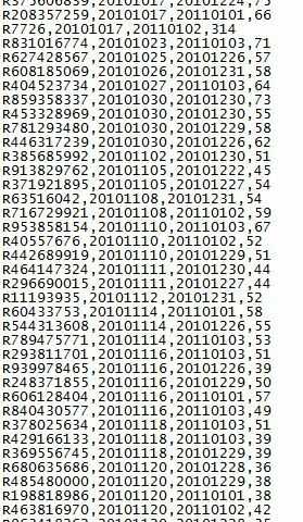
Everyday I download data from a site that will have rows each filled with individual data for clients. I'm able to input the data into excel as a whole but after that I'm having trouble figuring out how to put it into a chart.

For example Web visits time. So say Client 1 stayed for 5 min increasing his total time on the site to 20 min and Client 2 stayed for 0 min keeping his time of 10 min and they were both registered on new years eve, and R1's last login was today and R2's was yesterday. (R for some reason represents Client, no idea why...). Client 3 hasn't been on since he registered keeping his total at 4 min

So my data would look something like this for Today (20110104)

R1,20101231,20110104,20

R2,20101231,20110103,10

R3,20101231,20101231,4

And this for the day before (201101030),

R1,20101231,20110102,15

R2,20101231,20110103,10

R3,20101231,20101231,4

I get about 200+ client rows each day where even the names of the Client list are changing. Is it possible to import the data each day and fill it in a Excel sheet where the Client number is off on the left hand side in a table, and the amount of time (Whole Number ex. 4) each day it spends on the site extend to the right under it's specific date see Picture?

I've managed to create a manual sheet but have been unsuccessful at getting Excel to do any of it for me.

Here are two pictures:

One thought process of how it could be done is to create a macro prompting for the csv file, then for each client, find it, subtract the new total minutes with the previous total minutes (say 22 - 18 = 4), insert the difference into today's column. Then delete all the zero's in the range. If the client is not found it could be skipped until all clients that are left are new users, then the table could be expanded downwards by the number of clients left. In those new spots the client # could be entered.

Answer 1

I'm not sure you can have this happen completely automatically short of writing an amazing script....but if you could do that I'd recommend writing a real program with a database. I digress.

I assume your left most column is a sum of all the other columns for a particular row. I'm confused by the different #'s for client. prefix, suffix, and then what's the number in orange at the top? I'll proceed assuming that each client is a different row.

First you need to put the new file in a worksheet (probably in the same file) so you can reference it.

Assuming you have some common ID between each file....you have to first add any new clients to your master list. Maybe do this manually. you can use a =countif(thisID, <range of known id's>) against each day's new file to see if there are new ones and which ones. Ones that have a 0 would be new. Or if the id's are in order and always adding to the bottom, you can just look at the biggest # on both lists and add to it if necessary.

Now that your list is whole, put a vlookup function in today's column. and subtract the the existing total minutes=vlookup(<cell with clientid>, <range from today's file including all columns>, 4, false) - A<samerow>.

(the "4" is supposed to give you the client's minutes, so if it's not, something's wrong)

So what you have now in this column is today's minutes. But because you'll do the same thing tomorrow, you have to remove teh formula and replace it with actual values so they don't change later. So copy the whole column, then paste over it by right clicking, selecting 'paste special..." and chose "values".

That should get you pretty close to what you need with hopefully a few less steps. Sorry if that's not what you were looking for. Good luck!