Use Excel formulae results in array for nested function

In Excel, is it possible to have multiple formulae slot together into an array for a nested function?

Consider

=SMALL({10\15\20\25\30},1)

The formula returns the smallest value in the array. Now I'm trying to do something similar but not with a static array but something like this:

=SMALL({VLOOKUP($A$1,$A$2:$C$11,2)\VLOOKUP($A$1,$A$2:$C$11,3)\VLOOKUP($A$1,$A$2:$C$11,4)},1)

But that does not work unfortunately.

SilentRevolution

Posted 2018-01-28T17:03:54.263

Reputation: 93

Google array formula – I say Reinstate Monica – 2018-01-28T17:15:38.297

1Why don't you use min? =min(VLOOKUP($A$1,$A$2:$C$11,2),VLOOKUP($A$1,$A$2:$C$11,3),VLOOKUP($A$1,$A$2:$C$11,4)) – Máté Juhász – 2018-01-28T17:15:41.380

@TwistyImpersonator I did look at that but it was still unclear to me if I could combine function results in an array for further calculation. – SilentRevolution – 2018-01-28T19:28:09.177

@MátéJuhász actually for the time being that is good solution, thank you! – SilentRevolution – 2018-01-28T19:36:14.157

Answers

Your first formula works because it is using an array constant properly.

An array constant is a simple list of numbers or strings enclosed in curly brackets like:

 {1,2,3,4}

The following expressions will not work:

{1,2,3,4+1}
{A1,B3,C9}
{SUM(A1:B9),SUM(T7:T9)}

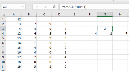
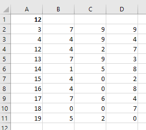
So if we have:

and we want to use SMALL() then enter:

=VLOOKUP($A$1,$A$2:$D$11,2,FALSE)
=VLOOKUP($A$1,$A$2:$D$11,3,FALSE)
=VLOOKUP($A$1,$A$2:$D$11,4,FALSE)

In F4 through H4 respectively and then we can use:

=SMALL(F4:H4,1)

Gary's Student

Posted 2018-01-28T17:03:54.263

Reputation: 15 540

I see, This is quite unfortunate as I was hoping to combine INDEX to find all instances of an item in a table and return the corresponding components required, to feed a VLOOKUP to to find component requirement and availability for an item and determine how many items can be built depending on the constraining component availability. But as demonstrated by you, this seems impossible without a step in between. – SilentRevolution – 2018-01-28T19:38:26.447

@SilentRevolution Good Luck! – Gary's Student – 2018-01-28T19:44:29.057

1Thanks, I already have the {=ROUNDDOWN(VLOOKUP(INDEX(ComponentRequirement;SMALL(IF(ComponentRequirement[Type]=[@Type];ROW(ComponentRequirement[Type]));1)-31;2);ComponentAvailability;3;FALSE)/INDEX(ComponentRequirement;SMALL(IF(ComponentRequirement[Type]=[@Type];ROW(ComponentRequirement[Type]));1)-31;3);0)} which finds the first, component (change k in the SMALL to find component 2 and 3), and that could feed into the table, in columns Component1\Component2\Component3 and then use the three cells for the last SMALL Function to find the constraining component. – SilentRevolution – 2018-01-28T19:53:11.913

You can use an array constant in place of the VLOOKUP column index number, e.g.

=SMALL(VLOOKUP($A$1,$A$2:$D$11,{2\3\4}),1)

This is an "array formula" that needs to be confirmed with CTRL+SHIFT+ENTER

Another way with INDEX and MATCH.....

=SMALL(INDEX($B$2:$D$11,MATCH($A$1,$A$2:$A$11),0),1)

Needs just "normal" entry

barry houdini

Posted 2018-01-28T17:03:54.263

Reputation: 10 434