Average by month within multiple bespoke date ranges excel

Question

I have data by month from January 2013 -> October 2017 as such

MONTH   MY DATA
Jan-13  45.0
Feb-13  23.0
.   
.   
.   
Oct-17  98.4

I wish to average data by calendar month, for specific, non-contiguous date ranges. E.G. January 2013 - > March 2013 and October 2016 -> May 2017.

I believe this can be accomplished by using IF functions with OR, to encompass multiple date ranges, and AND, to encompass two dates within each range, to return an array (when entering as an array formula) then using averageif on the returned array.

With my data in B5:C62 and my bespoke date ranges set up as:

Period 1 Start: S2
Period 1 End: T2
Period 2 Start: S3
Period 2 End: T3

And my calendar months in P6:P17, I enter my formula as

=AVERAGEIF($B$5:$B$62,P6,IF(OR(AND($B$5:$B$62>=$S$2,$B$5:$B$62<=$T$2),
AND($B$5:$B$62<=$S$3,$B$5:$B$62>=$T$3)),$C$5:$C$62,"ERROR"))

I get a #VALUE! error, though I can't see why. As far as I can tell my IF clause should be returning the "average_range" for the AVERAGEIF formula to run on.

What is the error in my formula or my approach?

Answer 1

In your formula, the IF() portion won't return an array when there is an AND() as part of the logical test. You can check this by using the built-in debugging tool for Excel formulas: highlight a portion of the formula in the formula bar and hit F9.

But there IS a way to calculate the average you want. In Excel, multiplying logical values converts True/False values into 1's and 0's, which can then be manipulated further. As an example, this statement

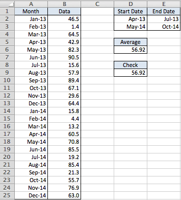
=(A2:A25>=D2)*(A2:A25<=E2)+(A2:A25>=D3)*(A2:A25<=E3)

returns the array

{0;0;0;1;1;1;1;0;0;0;0;0;0;0;0;0;1;1;1;1;1;1;0;0}

from the data in the table below. Here the multiplication acts like a logical AND and the addition is almost like a logical OR. (@Máté Juhász may chime in here to explain why it's not quite an OR :-)

This array can be viewed as a "mask" of column A with 1's corresponding to the two date ranges specified by the start and end dates.

Now an IF() formula can use this array to generate the list of values that you want to average:

IF(((A2:A25>=D2)*(A2:A25<=E2)+(A2:A25>=D3)*(A2:A25<=E3)),B2:B25)

This gives the array

{FALSE;FALSE;FALSE;42.9;82.3;90.5;15.6;FALSE;FALSE;FALSE;FALSE;FALSE;FALSE;FALSE;FALSE;FALSE;70.8;85.5;19.2;85.4;21.3;55.7;FALSE;FALSE}

which can now be fed to AVERAGE().

So one solution to your problem is a formula similar to this (array) formula, in D6:

=AVERAGE(IF(((A2:A25>=D2)*(A2:A25<=E2)+(A2:A25>=D3)*(A2:A25<=E3)),B2:B25))

Change the ranges and bespoke date values to fit your situation.

The cell below "Check" just contains a manual calculation of the average using

=AVERAGE(B5:B8,B18:B23)

Hope this helps and good luck.