6
0
The problem I'm essentially trying to solve is a VLOOKUP that is checking Columns A:E for a value, and returning the value held in Column F should it be found in any of these.
With VLOOKUP not being up to the task I have looked into the INDEX-MATCH syntax, but I am struggling to get my head around how to complete this for an array of values, as opposed to a single column. I've built an example data set below to try and explain this:
A------B------C------D------E------F

1------2------3------4------5------Apple

12-----13--------------------------Banana

14---------------------------------Carrot
Should the cell being checked contain 1,2,3,4 or 5, the result of the formula should be Apple. If it is 12 or 13, it should return Banana and finally if it contains 14, it should return Carrot.
The second half to this comes from the fact that the cell being referenced isn't a single value, but a full table itself. As such, this search will be completed a large number of times according to different values.
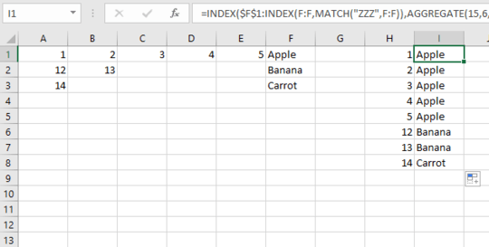
So to demonstrate, there is another table elsewhere (as below) that has these values in. I am attempting to have the system identify which row, and therefore which of the "Apple, Banana, Carrot" values to associate with each column. The table would look as below
H------I------------
1------(Apple)----
2------(Apple)----
12-----(Banana)-
etc.-----------------
The values in brackets are where the formula is calculating these values.


1Try this non array formula, it combine yours into one formula and deals with duplicates by finding the first row with that number;
=IFERROR(INDEX($F$1:$F$3,MIN(IFERROR(MATCH($H1,A$1:A$3,0),9999),IFERROR(MATCH($H1,B$1:B$3,0),9999),IFERROR(MATCH($H1,C$1:C$3,0),9999),IFERROR(MATCH($H1,D$1:D$3,0),9999),IFERROR(MATCH($H1,E$1:E$3,0),9999))),"")– Scott Craner – 2016-05-18T14:42:59.113If you ever get above row 9999 then you will need to increase that number, I just did not want to type
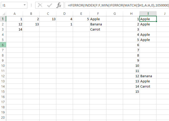
10500005 times, but that would allow you to use full column references, if you did. – Scott Craner – 2016-05-18T14:44:35.2031Here is the full column reference formula:
=IFERROR(INDEX(F:F,MIN(IFERROR(MATCH($H1,A:A,0),1050000),IFERROR(MATCH($H1,B:B,0),1050000),IFERROR(MATCH($H1,C:C,0),1050000),IFERROR(MATCH($H1,D:D,0),1050000),IFERROR(MATCH($H1,E:E,0),1050000))),"")– Scott Craner – 2016-05-18T14:47:17.907I edited my answer to show. – Scott Craner – 2016-05-18T14:49:42.843
It looks like your formula does a great job of combining these together - hard to judge the level to which it has sped things up as it seems to be roughly equivalent at this stage. Prevents the need for my array of values though. – Richard Allan – 2016-05-19T09:42:28.613