Excel: conditional formatting with with complex function AND

Question

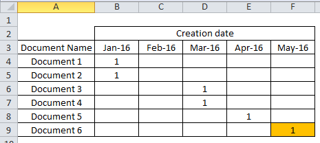
I have a sheet that looks like this:

So I have a list of documents to create, and I mark "1" on the column with the month in which I have created them.

Now I've been asked to put "1" also as a forecast documents not yet created, and these should be painted yellow. The sheet is actually huge and I wanted to automate it. I tried the Conditional Formatting using the formula:

=AND(B4>0;MONTH(B$3)>MONTH(TODAY());YEAR(B$3)>YEAR(TODAY())) 

Which works fine for the cell B4, but when I drag it over the sheet the formula doesn't automatically adjust. Does anyone have a clue about it? Or maybe a link to another topic about it?

Answer 1

So, the first problem with the formula is that it requires serial number of the month and the year of the Creation Date to be greater than the serial number and year of the current date. This will result in cells in the future not being highlighted. For example, 1/1/17 has a month number of 1 and 4/14/16 has a month number of 4. A 1 in the Jan-17 column would not be highlighted even though it is in the future because 1 is less than 4.

As long as the dates you used in row 3 are all the first day of the month (e.g. Jan-16 = 1/1/2016, Feb-16 = 2/1/2016), you can use the below formula.

=AND(B$3>TODAY(),B4>0)