Retrieve the array indexes from a range

I am facing an issue where I need to input column indexes from 1 to 1220 in the VLOOKUP function

{=SUM(VLOOKUP(A2,sheet1!$A$3:$AC$11, {1,2, 3, 4, 5, 6, ..., 1219, 1220}, TRUE))}

The only solution I see for that is to write a VBA function which will take a range and return an array of integers, but I need to avoid sending an Excel file with macros.

Is there any other possible way, solely based on Excel functions?

sheet example:

enter image description here

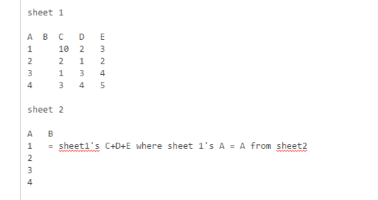
I need to match column A from sheet 2 with column A from sheet 1 then sum the rest of the row.

And it has to work as well if the sheet 2 is like the following:

Abdellah IDRISSI

Posted 2016-02-25T14:38:23.413

Reputation: 113

1While there might be a perfect answer to your question, can you give a little more context on what you're trying to do? There's also likely a better way to get what you want without using an array of integers. – Dane – 2016-02-25T14:45:37.160

Since you're using TRUE with VLOOKUP(), are you not expecting an exact match? – Kyle – 2016-02-25T14:59:26.427

As @Dane has said, this is a classic case of an XY Problem. Let us know your actual requirement for this formula - it looks like you're simply trying to add all the values on a row where A2 roughly matches the first column...?

– Jonno – 2016-02-25T15:01:37.753

@Jonno, yes that's what I am trying to achieve – Abdellah IDRISSI – 2016-02-25T15:07:36.953

@Skyline Please can you provide a sample of data, so we know what you're trying to match? Using TRUE with vlookup always seems fairly unpredictable when I've used it before. – Jonno – 2016-02-25T15:20:02.583

@Jonno I edited the question in order to provide the sample – Abdellah IDRISSI – 2016-02-25T15:36:32.420

Answers

Using your sample data (Note - I've mixed up row 2 and 3 so you can see they're performing a lookup, not just assuming positions):

The formula:

=SUM(INDEX(Sheet1!C:XFD,MATCH(A1,Sheet1!A:A,0),0))

This adds up all columns from C to XFD (The last possible column in Excel 2007+), by finding the row matching A1 in the column A of Sheet1.

Jonno

Posted 2016-02-25T14:38:23.413

Reputation: 18 756

Does this still work if the sheet 2 is this way http://i.stack.imgur.com/YNCby.png

– Abdellah IDRISSI – 2016-02-25T16:19:44.193

@Skyline I'm having trouble understanding exactly what you want. Can you try the formula and let me know if it doesn't work as expected, and how it should behave if it doesn't? – Jonno – 2016-02-25T16:22:43.170

the behavior of the formula you wrote is exactly what I want, but it doesn't work if the sheet 2 is like this http://i.stack.imgur.com/YNCby.png

– Abdellah IDRISSI – 2016-02-25T16:24:36.717

@Skyline http://imgur.com/tkSOpTG.jpg ?

– Jonno – 2016-02-25T16:40:25.990

That will work, but if you modify the column A, to be like the picture I sent, it will no longer work, VLOOKUP works in that case but it needs to be provided with column indexes. – Abdellah IDRISSI – 2016-02-25T17:00:16.390

@Skyline I'm still confused by what you mean - do you mean using values 1, 3 and 6? Where 6 will show #N/A because there isn't a 6? – Jonno – 2016-02-25T17:04:24.250

Sorry, 6 was just an example, here is the expected behavior http://imgur.com/Mx78Md6

– Abdellah IDRISSI – 2016-02-25T17:13:22.567

@Skyline This is why I'm confused - As far as I can tell, that's exactly what my formula is doing? http://i.imgur.com/oCIyFnA.jpg

– Jonno – 2016-02-25T17:17:24.720

here is what I am given when I try your formula http://imgur.com/mwjOVr6

– Abdellah IDRISSI – 2016-02-25T17:27:34.433

I can see that you mixed up the values on the sheet, but it was done on the wrong sheet – Abdellah IDRISSI – 2016-02-25T17:28:18.860

@Skyline You've changed the formula? =SUM(INDEX(Sheet! C1:E1 , MATCH(A1,Sheet1!A1:A4,0),0)) of course won't work, the match will find the row the data is on, but the index isn't being given that row. Change it back to C:XFD, or atleast specify C1:E99999 or something... – Jonno – 2016-02-25T17:36:14.217

this is the behavior I get when I use the same exact formula http://imgur.com/mdh45qc

– Abdellah IDRISSI – 2016-02-25T17:52:06.287

C:XFD ends up with C being quoted and has the same behavior.. – Abdellah IDRISSI – 2016-02-25T17:53:21.747

I'm using excel 2016. – Abdellah IDRISSI – 2016-02-25T17:55:57.543

@Skyline I'm not really sure what else to suggest - I'm also using Excel 2016 and just copy and pasted the formula back in without a problem. Sorry. – Jonno – 2016-02-25T17:57:20.833

I was using excel in compatibility mode (2003), since the excel file is gonna be used on that version of excel, I've tried your formula on a new excel file without compatibility mode and it works. – Abdellah IDRISSI – 2016-02-25T18:21:10.707

1@Skyline Glad you found the cause. For future questions, make sure you include your initial problem as well as all the factors that may influence a solution. In this instance, you can't actually have 1200 columns for a compatible spreadsheet, 256 would have been the limit. – Jonno – 2016-02-26T05:04:08.490

1200 was just for the example as well, the cell limit didn't match it "$AC", though thanks a lot for the help, and I will provide better information for future issues. – Abdellah IDRISSI – 2016-02-26T06:14:50.137

Instead of typing out {1,2,3,...,1220}, use ROW(A$1:A$1220), so using your example, your formula looks like:

=SUM(VLOOKUP(A2,sheet1!$A$3:$AC$11,ROW(A$1:A$1220),TRUE))

Note: This formula returns an error, because A3:AC11 does not contain 1220 columns.

Kyle

Posted 2016-02-25T14:38:23.413

Reputation: 2 286