The Search for a Search - Measuring the Information Cost of Higher Level Search/Critique of the Draft
The following is a critique of a previous draft of the paper. Some of the problems mentioned here were rectified, others seems to be still there...
| Original Text | Annotations |
|---|---|
|
Abstract—Many searches are needle-in-the-haystack problems, looking for small targets in large spaces. In such cases, blind search stands no hope of success. Success, instead, requires an assisted search. But whence the assistance required for a search to be successful? To pose the question this way suggests that successful searches do not emerge spontaneously but need themselves to be discovered via a search. The question then naturally arises whether such a higher-level “search for a search” is any easier than the original search. We prove two results: (1) The Horizontal No Free Lunch Theorem, which shows that average relative performance of searches never exceeds unassisted or blind searches. (2) The Vertical No Free Lunch Theorem, which shows that the difficulty of searching for a successful search increases exponentially compared to the difficulty of the original search. |
The idea of the annotations is to show the problems in this article of Dembski and Marks, problems which seem to lead to a erroneous formulation of the Horizontal No Free Lunch Theorem and a fault in its proof. An example ( Shell Game ) is constructed on which Dembski's and Marks's theorem doesn't work. |
|
Index Terms — No Free Lunch Theorems, active information, active entropy, assisted search, endogenous information |
Section I. Introduction (annotated)
| Original Text | Annotations |
|---|---|
| Conservation of information theorems [15], [44], especially the No Free Lunch Theorems (NFLT’s) [28], [51], [52], show that without prior information about the search environment or the target sought, one search strategy is, on average, as good as any other. | There is a condition for a search-strategy in the No Free Lunch Theorems to be on average, as good as any other: it has to be a search without repetition. The original paper are quite explicit in this regard, and it seems to be clear - you can construct a worse search by looking at the same place each time. So, though this seems to be obvious, it is a crucial point for the evaluation of the paper of Marks and Dembski. |
| Accordingly, the difficulty of an unassisted—or blind—search problem [9] is fixed and can be measured using what is called its endogenous information. | What is called endogenous information? This should read: what Marks and Dembski call endogenous information..., as they invented this phrase in their previous paper. For a finite search space Ω and a subset T - the target - this is  , generally it's the negative of the logarithm of the probability to find your target in a single guess. , generally it's the negative of the logarithm of the probability to find your target in a single guess. |
| The amount of information externally introduced into an assisted search can then be measured and is called the active information of the search [33]. Even moderately sized searches are virtually certain to fail in the absence of information concerning the target location or the search space structure. Knowledge concerning membership in a structured class of problems, for example, can constitute search space structure information [50]. | It isn't directly measured, it's more the other way round: For a succesful search, Dembski and Marks define the active information as the endogenous information.... |
|
Endogenous and active information together allow for a precise characterization of the conservation of information. |
... at least in the sense that for a successful search, the endogenous information at the beginning of the search equals exactly - but not surprisingly - the active information at its end... |
| The average active information, or active entropy,of an unassisted search is zero when no assumption is made concerning the search target. If any assumption is made concerning the target, the active entropy becomes negative. This is the Horizontal NFLT. It states that an arbitrary search space structure will, on average, result in a worse search than assuming nothing and simply performing an unassisted search. | This active entropy is quite a strange animal and will be defined in this article. The conclusion of the Horizontal NFLT seems to be wrong, and the failure in its reasoning will be discussed later. |
| The Horizontal NFLT addresses how changing a search space structure affects average search performance, but it does not address the difficulty of finding a search capable of locating a particular target. That is the job of the Vertical NFLT, which characterizes the information costs of searching higher-level search spaces for successful lower-level searches. Such higher-level searches are amenable to the same endogenous/active information analysis as lower-level searches. | The Vertical NFLT won't be discussed here. |
| As one might expect, no active information in the “search for a search” translates to zero active information in the lower-level search (which means that, on average, the lower-level search so found cannot do better than an unassisted search). This result holds for still higher level searches such as a “search for a search for a search” and so on. Thus, without active information introduced somewhere in the search hierarchy, none will be available for the original search. If, on the other hand, active information is introduced anywhere in the hierarchy, it projects onto the original search space as active information. |
|
Consider therefore the minimally acceptable active information required for a successful search. In searching for such a search, a higher-level search will need to introduce a certain amount of active information. How much? According to the Vertical NFLT, the cost of this higher-level active information increases exponentially with respect to the active information required in the lower-level search space. The Vertical NFLT therefore reveals that a “search for a search” yielding minimally acceptable active information in the original search space is a much more difficult problem than simply searching the original space directly. Based on computational difficulty, one should therefore generally choose an arbitrary unassisted search over “searching for a good search.” |
That sounds - well - absurd at first. For a successful search, the minimally acceptable active information is the whole endogenous information, by definition... |
Section II. Information in Search (annotated)
| Original Text | Annotations |
|---|---|
| All but the most trivial searches require information about the search environment (e.g., smooth landscapes) or target location (e.g., fitness measures) if they are to be successful. Conservation of information theorems [15], [28], [44], [51], [52] show that one search algorithm will, on average, perform as well as any other and thus that no search algorithm will, on average, outperform an unassisted, or blind, search. But clearly, many of the searches that arise in practise do outperform blind unassisted search. How, then, do such searches arise and where do they obtain the information that enables them to be successful? | In fact, only the most trivial search (Searching for the haystack in a haystack) requires no fitness measures. At least, if you care for a successful search. |
A. Unassisted Search
| Original Text | Annotations |
|---|---|
| Exhaustive search, random sampling, random walks, and searches along Brownian motion paths all exemplify blind search, a.k.a. unassisted search. In a blind or unassisted search, no prior information concerning the location of the target or the structure of the search space is available. Such a search therefore assumes a uniform probability distribution on the search space. Given any knowledge about the target location or the search space structure constitutes information and voids this assumption [33]. | Random walks and searches along Brownian motion do assume prior information of the structure of the search space: you have to have a concept of neighbours, or nearness, i.e., some (not discrete!) metric. |
| For example, given a deck of 52 cards face down and the task of choosing the A♠, and given no information about the location of the cards or how they are laid out, one rightly assumes each card has the same probability of turning up the A♠. This uniformity assumption is Bernoulli’s principle of insufficient reason, which states that in the absence of any prior information, “we must assume that the events ... have equal probability” [2], [36]. Uniformity is equivalent to the assumption that the search space is at maximum informational entropy. | Wow, nothing wrong here! Minor beef: The references - Bernoulli's ars coniectandi - that's utterly pretentious. And the second one, Papoulis's Probability, Random Variables, and Stochastic Processes hints to pages 537-542 - again - where you find nothing about an uniformity assumption. |
B. Assisted Search
| Original Text | Annotations |
|---|---|
| De?ne an assisted search as any procedure that provides more information about the search environment or candidate solutions than a blind search. The classic example of an assisted search is the Easter egg hunt in which instead of saying “yes” or “no” to a proposed location where an egg might be hidden, one says “warmer” or “colder” as distance to the egg gets smaller or bigger. This additional information clearly assists those who are looking for the Easter eggs, especially when the eggs are well hidden and blind search would be unlikely to ?nd them. Information about a search environment can also assist a search. A maze that has a unique solution and allows only a small number of “go right” and “go left” decisions constitutes an information-rich search environment that helpfully guides the search. | Just to stress a point: the Easter eggs are hidden first, then searched. They don't pop up somewhere during the search - or magically change their position. That's a search as it is generally understood. Of course, there is nothing wrong with a moving target: But you should say so if you are looking for one. Or when you change the rules of the search: for instance, if you expect that an egg is found at each step of the process (quite absurd, isn't it?) |
Suppose now denotes an arbitrary search space. In general, assume is a compact metric space with metric D, though for most theorems and calculations assume is finite (in which case D is a discrete metric). Let  denote denote  -valued random variables that are independent and identically distributed with uniform probability distribution U. therefore represents a blind search of . Next, -valued random variables that are independent and identically distributed with uniform probability distribution U. therefore represents a blind search of . Next,  denote denote  -valued random variables that are arbitrarily distributed. therefore characterizes an assisted search of . -valued random variables that are arbitrarily distributed. therefore characterizes an assisted search of . |
Just checking: is a search for the target  . When is such a search a success? If . When is such a search a success? If  for one for one  . How many possible targets are there? . How many possible targets are there?  . . |
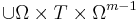
If we now let  denote the m-fold Cartesian product of denote the m-fold Cartesian product of  , then , then  and and  are m-valued random variables. Because the uniform probability on m is just the m-fold product measure of U [11], is uniformly distributed on are m-valued random variables. Because the uniform probability on m is just the m-fold product measure of U [11], is uniformly distributed on  = . Thus, by attending solely to the probabilistic structure of searches, we represent the blind search = . Thus, by attending solely to the probabilistic structure of searches, we represent the blind search  := as having a m-dimensional uniform distribution with respect to a metric := as having a m-dimensional uniform distribution with respect to a metric  that suitably extends to the metric D on . Moreover, we represent the assisted search that suitably extends to the metric D on . Moreover, we represent the assisted search  := , in searching for an arbitrary subset := , in searching for an arbitrary subset  of , as having distribution of , as having distribution  on . on . |
And come the problem: Without any warning R. Marks and W. Dembski state that they are now looking at arbitrary subsets of . That's something different from everything they've done before! Until now, the search was for a fixed, unmoving subset of . So, what's a successful search for such a set? As above, it requires that
or that
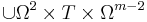
But most subsets of R. Marks and W. Dembski don't talk about a search with n steps any longer in any meaningful way, they are describing a one-step search in a bigger space, i.e., |
But all these tildes are superfluous. Dropping them, we see that the probabilistic connection between a blind search and an assisted search can be entirely characterized in terms of a search space , a metric D that induces a compact topology on , a target T included in , a uniform probability measure U on induced by D, and an arbitrary probability measure  on . U represents the probabilistic structure of a blind search, and represents the probabilistic structure of an assisted search. on . U represents the probabilistic structure of a blind search, and represents the probabilistic structure of an assisted search. |
Yes, you can drop the tildes. But you have to be careful. And the next paragraph shows that you are not... |
For convenience, we adopt the following notation (here “:=” indicates a definition):


 |
Here, the lack of the tildes add to the confusion. Do Marks and Dembski speak about the original search space  , or about the late ? One would expect that K is the size of the original space, but that p and q are calculated in the world of tildes... , or about the late ? One would expect that K is the size of the original space, but that p and q are calculated in the world of tildes... |

 .
. :
:
 implies that
  for all
  to
to  , and for a success, you have to hit it at each step! That's no search, that's playing whac-a-mole with a blindfold on.
Section III. Active Information and no Free Lunch (annotated)
| Original Text | Annotations | ||||||||||||||||||||||||||||||||||||||||||||||||||||||
|---|---|---|---|---|---|---|---|---|---|---|---|---|---|---|---|---|---|---|---|---|---|---|---|---|---|---|---|---|---|---|---|---|---|---|---|---|---|---|---|---|---|---|---|---|---|---|---|---|---|---|---|---|---|---|---|
Gauging the effectiveness of assisted search in relation to blind search is our next task. Random sampling with respect to the uniform probability U sets a baseline for the effectiveness of blind search. For a ?nite search space with K elements, the probability of locating the target T has uniform probability
 (III.1) (III.1) |
That's only true for a single guess... | ||||||||||||||||||||||||||||||||||||||||||||||||||||||
We assume that we can always do at least as well as uniform random sampling. The question is, how much better can we do? Given a small target T in and probability measures U and  characterizing blind and assisted search respectively, assisted search will be more effective than blind search just in case p < q, as effective if p = q, and less effective if p > q. In other words, an assisted search can be more likely to locate T than blind search, equally likely, or less likely. If less likely, the assisted search is counterproductive, actually doing worse than blind search. For instance, we might imagine an Easter egg hunt where one is told “warmer” if one is moving away from an egg and “colder” if one is moving toward it. If one acts on this guidance, one will be less likely to ?nd the egg than if one simply did a blind search. Because the assisted search is in this instance misleading, it actually undermines the success of the search. characterizing blind and assisted search respectively, assisted search will be more effective than blind search just in case p < q, as effective if p = q, and less effective if p > q. In other words, an assisted search can be more likely to locate T than blind search, equally likely, or less likely. If less likely, the assisted search is counterproductive, actually doing worse than blind search. For instance, we might imagine an Easter egg hunt where one is told “warmer” if one is moving away from an egg and “colder” if one is moving toward it. If one acts on this guidance, one will be less likely to ?nd the egg than if one simply did a blind search. Because the assisted search is in this instance misleading, it actually undermines the success of the search. |
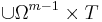
... but the Easter egg example indicates that Dembski and Marks aren't talking about a single guess, they are talking about a search, i.e., a sequence of guesses. So, what's the difference? Look at the original search, a sequence of -valued random variables  , looking for a non-empty subset T of . Define , looking for a non-empty subset T of . Define  as 1, if as 1, if  and 0 if and 0 if  . The search is a success, if . The search is a success, if
 . .Now, take the set  . .That's a bit of a difference! As stated earlier, to represent a search in the original space in | ||||||||||||||||||||||||||||||||||||||||||||||||||||||
|
An instructive way to characterize the effectiveness of assisted search in relation to blind search is with the likelihood ratio |
An example: Shell Game
Imagine a shell game. Three shells, and one, two or even three peas. Then Then
There are Let's look at two strategies:
Both strategies induce a measure on
Following the traditions of the No Free Lunch Theorems, the average is taken by assuming that all nonempty subsets T are equally likely to be searched for. We see that clever search fares better on average than uniform search when looking at the original problem. But that's not what W. Dembski and R. Marks are doing. In fact, they look at all subsets That's what all of R. Marks's and W. Dembski's idea is about: on average, our clever search does as good - or as bad - as the uniform search. But that's nonsense: Most of the subsets of But what if we look only at subsets Then we get a problem in the next section: For the formulation and the proof of their Horizontal No Free Lunch theorem, a partition of |
 in
in  in
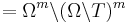
in  is a success if
  . So no harm done, just use sets having this special structure. Unfortunately, it isn't that easy: Dembski's and Marks's assumptions need to look at other sets...
 (we always assume p > 0). This ratio achieves a maximum of
  when q = 1, in which case the assisted search is guaranteed to succeed. The assisted search is better at locating T than blind search provided the ratio is bigger than 1, equivalent to blind search when it is equal to 1, and worse than blind search when it is less than 1. Finally, this ratio achieves a minimum value of 0 when q = 0, indicating that the assisted search is guaranteed to fail.
 - the three shells. And there are
  non-empty subsets of

 .
.  non-empty subsets of
  ...
... in
in 


 . Taking into account the special case of
  , you get the number...)
 . According to Marks and Dembski, the search is successful if you get that the pea is under shell 3 in your first try and that is under shell 2 or under shell 1 in your second try. Finding it once isn't enough! Of course, clever search get this wrong: Though it looks under shell 2 in the second step - and finds a pea - it has failed to find a pea in the first attempt, consistent with
  . A uniform search may look under shell 3 the first time, and shell 2 or 1 the second time - U({(3,2),(3,1)}= 2/9. But that's no search any longer - we're dealing with a guess, a guess on more complicated spaces.
A. Active Information
| Original Text | Annotations |
|---|---|
De?ne the active information of an assisted search as
   When the target T is clear from context, we suppress the superscript T and simply write |
Have a look at our example: For  , this leads to , this leads to A-ha... That's less than the weight of the sun in grams... |
| Active information measures the effectiveness of assisted search in relation to blind search using a conventional information measure. It [33] characterizes the amount of information [8] that (representing the assisted search) adds with respect to U (representing the blind search) in the search for T. Active information therefore quantifies the effectiveness of assisted search against a blind-search baseline. The NFLT dictates that any search without active information will, on average, perform no better than blind search. This baseline may therefore be properly interpreted as holding for arbitrary searches in general and not just for blind search. |
The blind search of the NFLT is by the way not the uniform search of R. Marks and W. Dembski: it explicitly is a search without repetition, i.e., if  is a realization of a blind search in the sense of the NFLT for a subset T of Ω, then is a realization of a blind search in the sense of the NFLT for a subset T of Ω, then  . Furthermore, the phrase active information doesn't occur in the original works on the NFLT... . Furthermore, the phrase active information doesn't occur in the original works on the NFLT... |
The maximum value that active information can attain is  indicating an assisted search guaranteed to succeed (i.e. a perfect search) [33]); and indicating an assisted search guaranteed to succeed (i.e. a perfect search) [33]); and
the minimum it can attain is |
Now, some new concepts are introduced. We'll stick to our example and have a look at and its corresponding set  , as well as an arbitrary set , as well as an arbitrary set  |
|
In the difference  (III.3) (III.3)Endogenous information represents the fundamental difficulty of the search in the absence of any external information. Like other log measurements (e.g., dB), the active information in (III.3) is measured with respect to a reference point. Here endogenous information based on blind search serves as the reference point. |
|
The endogenous information bounds the active information in (III.3).
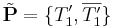
  if the assisted search is guaranteed never to succeed. if the assisted search is guaranteed never to succeed. |
And indeed,  , as this search never succeeds to find , as this search never succeeds to find  . But why should it? . But why should it? |
The second term in (III.3), is the exogenous information.
 (III.4) (III.4)
|
 , ,  |
|
Active information as defined in (III.3) could also be measured with respect to other reference points. We therefore define the active information more generally as   (III.5) (III.5)for |
Impressive, but usually we're only concerned with finite sets, discrete metrics, etc. Seems to be difficult enough to get that math right... |
 instead of
  . (likewise, for the endogenous information
  and the exogenous information
  — see below — we write
  and
and  when T is clear).
 , indicating an assisted search guaranteed to fail.
 , we call the first term the endogenous information.
 .
.B. Horizontal No Free Lunch
| Original Text | Annotations |
|---|---|
|
Since the mid-1990s, several conservation of information theorems for search have been proved [15], [28], [44], [51], [52]. The upshot of these theorems — also known as No Free Lunch (NFL) theorems — is that even though a given search may outperform other searches for specific targets, when averaged over the distinct ways searches may differ, no search outperforms any other. Thus, in particular, random search, on average, performs as well as any other. The following No Free Lunch theorem (NFLT) underscores this parity of average search performance. |
Now, we come to the core of the problem |
|
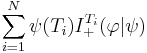
Theorem III.1. Horizontal No Free Lunch. Let
Then |
Wow, that's a mouthful. First  should be should be  , but that doesn't really matter. The problem is the partition, which is inconveniently named , again. So, to reduce confusion, we'll talk about the partition P. Let's see how this works on our example, taking as the measure linked to our clever search, i.e, , but that doesn't really matter. The problem is the partition, which is inconveniently named , again. So, to reduce confusion, we'll talk about the partition P. Let's see how this works on our example, taking as the measure linked to our clever search, i.e,  , and as , and as  , the uniform measure U. , the uniform measure U.
To explain it with the example of our Easter egg hunt: if you think you have a clever algorithm to work for your egg hunt, you don't expect it to work when
But in the calculation of |
|
Proof: The expression in (III.6) is immediately recognized as the negative of the Kullback-Leibler distance [8]. Since the Kullback-Leibler distance is always
nonnegative, the expression in (III.6) does not exceed zero. Equality is achieved iff for each |
Impressing, elegant, inapplicable. |
|
Because the active entropy is strictly negative unless the two probability measures |
This idea is not only counter-intuitive, it seems to be wrong: yes, if you include sets which don't resemble a search into the calculation of your average, then the assisted search perform worse. But even our simple example has shown that this isn't true in the real world... |
|
Corollary III.1. Horizontal No Free Lunch: No Information Known. Given any probability measure on |
An example of: ex falsum quodlibet |
|
Remarks. If no information about a search exists, so that the underlying measure is uniform, then, on average, any other assumed measure will result in negative active information, thereby rendering the search performance worse than random search. |
|
|
Proof: Using  (III.6) (III.6)From Theorem III.1, the expression in (III-B) is nonpositive. ♦ |
A proof for a corollary? Seems to be more of a lemma, then. |
 be an exhaustive partition of
 (III.6)
 with equality if and only if
  for
for  .
. . Then, there is the selection of corresponding sets in
  . Plugging this into the formula for
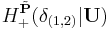
 . Why is this positive? Well,
  is no partition of
  So, this doesn't work as intended.
 and its complement in
  :
:  . Then
  . That's at least negative. But unfortunately, the set
  doesn't make sense in context of a search, and therefore, clever search shouldn't be used on it.
 .
.  ).Moreover, the degree to which it performs worse will track the degree to which the assisted search singles out and confers disproportionately high probability on only a few targets in the partition. This suggests that success of an assisted search depends on its attending to a few select targets at the expense of neglecting most of the remaining targets.
 and (III.1), the expression (III.6) in Theorem III.1 becomes
Section IV The Search for a Good Search
Just a short summary of a further problem: In this section, a probabilistic hierarchy on top of is introduced:  is the collection of all probability measures on . It is claimed (and hopefully proven) that is itself a compact metric space with Borel sets, so the process can be reiterated to get
  and so on. Define for convenience
  ,
,  ,
,  , and voilà, you have quite something!
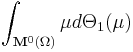
Now, an important integral is introduced to link the different spaces  : For an arbitrary probability measure
  on
on  (and therefore
  ), define

.
This is a vector-valued integration and no less than three references are given for it:
- Nicolae Dinculeanu, Vector Integration and Stochastic Integration in Banach Spaces, New York: Wiley, (2000)
- I. M. Gelfand, Sur un Lemme de la Theorie des Espaces Lineaires, Comm. Inst. Sci. Math. de Kharko. 13(4) (1936): 35–40.
- B. J. Pettis, On Integration in Vector Spaces, Transactions of the American Mathematical Society 44 (1938): 277–304.
So, we're talking about Bochner integrals or even Pettis-Gelfand integrals. Very interesting stuff! Only one problem: Though Marks and Dembski undertook some pain to get the space right over which they are integrating, they have a problem with the function in this integral: The Bochner (and Pettis-Gelfand integral)  is defined for a function
  , where
  is a measure-space and
  is a Banach space, i.e., a complete normed vector space.
And though this works out for  , you get a problem for
  :
:
Example: Let be a deck of cards. can be seen as a discrete metric space. Let's try to calculate  for
for  being the uniform probability measure. Then


Conclusion
When W. Dembski and R Marks state their Horizontal No Free Lunch theorem, they talk about an exhaustive partition of Ω all of whose partition elements have positive probabilities. You can build a partition of Ω of elements of the form  only if
  .
.
In this case, the whole result is trivial: If you are allowed only one shot onto an unknown target, just shoot at random!
But for bigger m, i.e., searches as they are generally understood (and described in their paper as assisted searches), the theorem falls flat. And with it, the rest of the paper.


