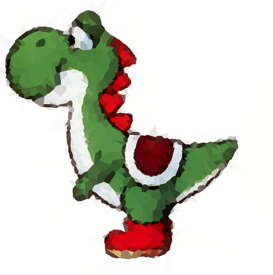
Draw an Image as a Voronoi Map

170

89

Credits to Calvin's Hobbies for nudging my challenge idea in the right direction.

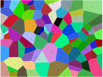
Consider a set of points in the plane, which we will call sites, and associate a colour with each site. Now you can paint the entire plane by colouring each point with the colour of the closest site. This is called a Voronoi map (or Voronoi diagram). In principle, Voronoi maps can be defined for any distance metric, but we'll simply use the usual Euclidean distance r = √(x² + y²). (Note: You do not necessarily have to know how to compute and render one of these to compete in this challenge.)

Here is an example with 100 sites:
enter image description here

If you look at any cell, then all points within that cell are closer to the corresponding site than to any other site.

Your task is to approximate a given image with such a Voronoi map. You're given the image in any convenient raster graphics format, as well as an integer N. You should then produce up to N sites, and a colour for each site, such that the Voronoi map based on these sites resembles the input image as closely as possible.

You can use the Stack Snippet at the bottom of this challenge to render a Voronoi map from your output, or you can render it yourself if you prefer.

You may use built-in or third-party functions to compute a Voronoi map from a set of sites (if you need to).

This is a popularity contest, so the answer with the most net votes wins. Voters are encouraged to judge answers by

  • how well the original images and their colours are approximated.
  • how well the algorithm works on different kinds of images.
  • how well the algorithm works for small N.
  • whether the algorithm adaptively clusters points in regions of the image that require more detail.

Test Images

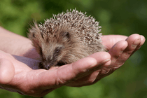
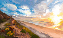
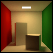
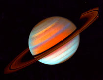
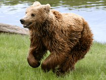
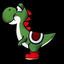
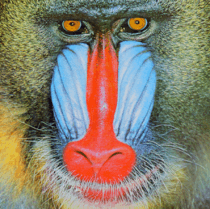
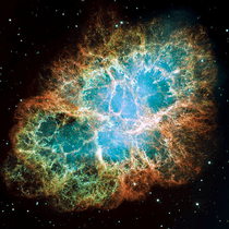
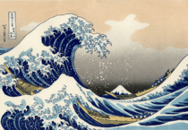
Here are a few images to test your algorithm on (some of our usual suspects, some new ones). Click the pictures for larger versions.

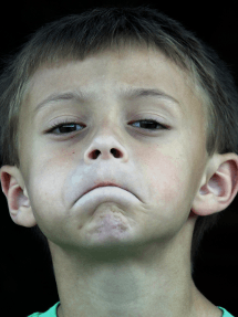
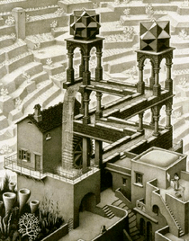
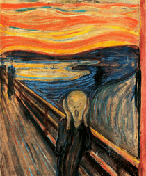
Great Wave Hedgehog Beach Cornell Saturn Brown Bear Yoshi Mandrill Crab Nebula Geobits' Kid Waterfall Scream

The beach in the first row was drawn by Olivia Bell, and included with her permission.

If you want an extra challenge, try Yoshi with a white background and get his belly line right.

You can find all of these test images in this imgur gallery where you can download all of them as a zip file. The album also contains a random Voronoi diagram as another test. For reference, here is the data that generated it.

Please include example diagrams for a variety of different images and N, e.g. 100, 300, 1000, 3000 (as well as pastebins to some of the corresponding cell specifications). You may use or omit black edges between the cells as you see fit (this may look better on some images than on others). Do not include the sites though (except in a separate example maybe if you want to explain how your site placement works, of course).

If you want to show a large number of results, you can create a gallery over on imgur.com, to keep the size of the answers reasonable. Alternatively, put thumbnails in your post and make them links to larger images, like I did in my reference answer. You can get the small thumbnails by appending s to the file name in the imgur.com link (e.g. I3XrT.png -> I3XrTs.png). Also, feel free to use other test images, if you find something nice.

Renderer

Paste your output into the following Stack Snippet to render your results. The exact list format is irrelevant, as long as each cell is specified by 5 floating point numbers in the order x y r g b, where x and y are the coordinates of the cell's site, and r g b are the red, green and blue colour channels in the range 0 ≤ r, g, b ≤ 1.

The snippet provides options to specify a line width of the cell edges, and whether or not the cell sites should be shown (the latter mostly for debugging purposes). But note that the output is only re-rendered when the cell specifications change - so if you modify some of the other options, add a space to the cells or something.

function draw() {
  document.getElementById("output").innerHTML = svg
}

function drawMap() {
  var cells = document.getElementById("cells").value;
  var showSites = document.getElementById("showSites").checked;
  var showCells = document.getElementById("showCells").checked;
  var lineWidth = parseFloat(document.getElementById("linewidth").value);
  var width = parseInt(document.getElementById("width").value);
  var height = parseInt(document.getElementById("height").value);
  var e = prefix.replace('{{WIDTH}}', width)
                .replace('{{HEIGHT}}', height);
  cells = cells.match(/(?:\d*\.\d+|\d+\.\d*|\d+)(?:e-?\d+)?/ig);
  var sitesDom = '';
  var sites = []
  for (i = 0; i < cells.length; i+=5)
  {
    x = parseFloat(cells[i]);
    y = parseFloat(cells[i+1]);
    r = Math.floor(parseFloat(cells[i+2])*255);
    g = Math.floor(parseFloat(cells[i+3])*255);
    b = Math.floor(parseFloat(cells[i+4])*255);
    sitesDom += '<circle cx="' + x + '" + cy="' + y + '" r="1" fill="black"/>';
    sites.push({ x: x, y: y, r: r, g: g, b: b });
  }
  
  if (showCells)
  {
    var bbox = { xl: 0, xr: width, yt: 0, yb: height };
    var voronoi = new Voronoi();
  
    var diagram = voronoi.compute(sites, bbox);
    for (i = 0; i < diagram.cells.length; ++i)
    {
      var cell = diagram.cells[i];
      var site = cell.site;
      var coords = '';
      for (var j = 0; j < cell.halfedges.length; ++j)
      {
        var vertex = cell.halfedges[j].getStartpoint();
        coords += ' ' + vertex.x + ',' + vertex.y;
      }
      var color = 'rgb('+site.r+','+site.g+','+site.b+')';
      e += '<polygon fill="'+color+'" points="' + coords + '" stroke="' + (lineWidth ? 'black' : color) + '" stroke-width="'+Math.max(0.6,lineWidth)+'"/>';
    }
  }
  if (showSites)
    e += sitesDom;
  e += suffix;
  e += '<br> Using <b>'+sites.length+'</b> cells.';
  svg = e;
  draw();
}
var prefix = '<svg width="{{WIDTH}}" height="{{HEIGHT}}">',
  suffix = "</svg>",
  scale = 0.95,
  offset = 225,
  radius = scale*offset,
  svg = "";
svg {
  position: relative;
}
<script src="http://www.raymondhill.net/voronoi/rhill-voronoi-core.js"></script>
Line width: <input id="linewidth" type="text" size="1" value="0" />
<br>
Show sites: <input id="showSites" type="checkbox" />
<br>
Show cells: <input id="showCells" type="checkbox" checked="checked" />
<br>
<br>
Dimensions: <input id="width" type="text" size="1" value="400" /> x <input id="height" type="text" size="1" value="300" />
<br>
Paste cell specifications here
<br>
<textarea id="cells" cols="60" rows="10" oninput='drawMap()'></textarea>
<br>
<br>
<div id="output"></div>

Massive credits to Raymond Hill for writing this really nice JS Voronoi library.
Related Challenges

Martin Ender

Posted 10 years ago

Reputation: 184 808

How do we verify we have done it the best way? – frogeyedpeas – 10 years ago

5

@frogeyedpeas By looking at the votes you get. ;) This is a popularity contest. There is not necessarily the best way to do. The idea is that you try to do it as well as you can, and the votes will reflect whether people agree that you've done a good job. There is a certain amount of subjectivity in these, admittedly. Have a look at the related challenges I linked, or at this one. You'll see that there is usually a wide variety of approaches but the voting system helps the better solutions bubble up to the top and decide on a winner.

– Martin Ender – 10 years ago

3Olivia approves of the approximations of her beach submitted thus far. – Alex A. – 10 years ago

3@AlexA. Devon approves of some of the approximations of his face submitted thus far. He's not a big fan of any of the n=100 versions ;) – Geobits – 10 years ago

1@Geobits: He'll understand when he's older. – Alex A. – 10 years ago

1Here's a page about a centroidal voronoi-based stippling technique. A good source of inspiration (the related master thesis has a nice discussion of possible improvements to the algorithm). – Job – 10 years ago

Did I make a comment about the use of the term "distance measure" and how it should be "metric" or am I going mental? I can't find the comment! – Alec Teal – 10 years ago

@AlecTeal You did, and I fixed it, and I replied... and I saw you were online since my reply, so I assumed you'd read it and deleted both comments as they were obsolete. ;) – Martin Ender – 10 years ago

I had linked to the definition because.... I have a maths background, but it might be the first time someone has seen a formal notion of "distance" and their "metrics" - that's why I included the link. You're using just 3 properties to generate this map. I am also quite interested in seeing what the pictures look like with different metrics.... http://www.maths.kisogo.com/index.php?title=Metric_space is the link BTW

– Alec Teal – 10 years ago

Is this just a puzzle or do you also think this could be an approach for a new type of compressed images? To me it looks like storing the coordinates and colors of the sites would need much less information than storing the image pixel by pixel. – Thomas Weller – 10 years ago

@ThomasWeller I just thought it's a fun challenge that is both challenging and would yield varied and interesting results. But the same thing has been discussed when I posted it in Hacker News, so maybe you can weigh in there.

– Martin Ender – 10 years ago

Answers

112

Python + scipy + scikit-image, weighted Poisson disc sampling

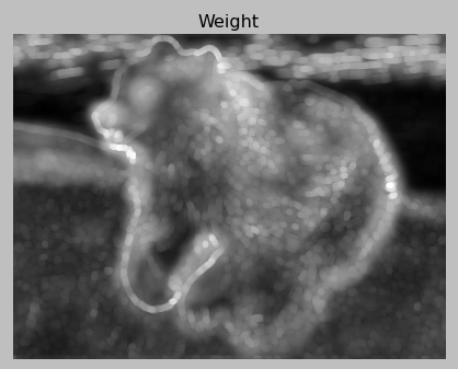
My solution is rather complex. I do some preprocessing on the image to remove noise and get a mapping how 'interesting' each point is (using a combination of local entropy and edge detection):

Then I choose sampling points using Poisson disc sampling with a twist: the distance of the circle is determined by the weight we determined earlier.

Then once I have the sampling points I divide up the image in voronoi segments and assign the L*a*b* average of the color values inside each segment to each segment.

I have a lot of heuristics, and I also must do a bit of math to make sure the number of sample points is close to N. I get N exactly by overshooting slightly, and then dropping some points with an heuristic.

In terms of runtime, this filter isn't cheap, but no image below took more than 5 seconds to make.

Without further ado:

import math
import random
import collections
import os
import sys
import functools
import operator as op
import numpy as np
import warnings

from scipy.spatial import cKDTree as KDTree
from skimage.filters.rank import entropy
from skimage.morphology import disk, dilation
from skimage.util import img_as_ubyte
from skimage.io import imread, imsave
from skimage.color import rgb2gray, rgb2lab, lab2rgb
from skimage.filters import sobel, gaussian_filter
from skimage.restoration import denoise_bilateral
from skimage.transform import downscale_local_mean


# Returns a random real number in half-open range [0, x).
def rand(x):
    r = x
    while r == x:
        r = random.uniform(0, x)
    return r


def poisson_disc(img, n, k=30):
    h, w = img.shape[:2]

    nimg = denoise_bilateral(img, sigma_range=0.15, sigma_spatial=15)
    img_gray = rgb2gray(nimg)
    img_lab = rgb2lab(nimg)

    entropy_weight = 2**(entropy(img_as_ubyte(img_gray), disk(15)))
    entropy_weight /= np.amax(entropy_weight)
    entropy_weight = gaussian_filter(dilation(entropy_weight, disk(15)), 5)

    color = [sobel(img_lab[:, :, channel])**2 for channel in range(1, 3)]
    edge_weight = functools.reduce(op.add, color) ** (1/2) / 75
    edge_weight = dilation(edge_weight, disk(5))

    weight = (0.3*entropy_weight + 0.7*edge_weight)
    weight /= np.mean(weight)
    weight = weight

    max_dist = min(h, w) / 4
    avg_dist = math.sqrt(w * h / (n * math.pi * 0.5) ** (1.05))
    min_dist = avg_dist / 4

    dists = np.clip(avg_dist / weight, min_dist, max_dist)

    def gen_rand_point_around(point):
        radius = random.uniform(dists[point], max_dist)
        angle = rand(2 * math.pi)
        offset = np.array([radius * math.sin(angle), radius * math.cos(angle)])
        return tuple(point + offset)

    def has_neighbours(point):
        point_dist = dists[point]
        distances, idxs = tree.query(point,
                                    len(sample_points) + 1,
                                    distance_upper_bound=max_dist)

        if len(distances) == 0:
            return True

        for dist, idx in zip(distances, idxs):
            if np.isinf(dist):
                break

            if dist < point_dist and dist < dists[tuple(tree.data[idx])]:
                return True

        return False

    # Generate first point randomly.
    first_point = (rand(h), rand(w))
    to_process = [first_point]
    sample_points = [first_point]
    tree = KDTree(sample_points)

    while to_process:
        # Pop a random point.
        point = to_process.pop(random.randrange(len(to_process)))

        for _ in range(k):
            new_point = gen_rand_point_around(point)

            if (0 <= new_point[0] < h and 0 <= new_point[1] < w
                    and not has_neighbours(new_point)):
                to_process.append(new_point)
                sample_points.append(new_point)
                tree = KDTree(sample_points)
                if len(sample_points) % 1000 == 0:
                    print("Generated {} points.".format(len(sample_points)))

    print("Generated {} points.".format(len(sample_points)))

    return sample_points


def sample_colors(img, sample_points, n):
    h, w = img.shape[:2]

    print("Sampling colors...")
    tree = KDTree(np.array(sample_points))
    color_samples = collections.defaultdict(list)
    img_lab = rgb2lab(img)
    xx, yy = np.meshgrid(np.arange(h), np.arange(w))
    pixel_coords = np.c_[xx.ravel(), yy.ravel()]
    nearest = tree.query(pixel_coords)[1]

    i = 0
    for pixel_coord in pixel_coords:
        color_samples[tuple(tree.data[nearest[i]])].append(
            img_lab[tuple(pixel_coord)])
        i += 1

    print("Computing color means...")
    samples = []
    for point, colors in color_samples.items():
        avg_color = np.sum(colors, axis=0) / len(colors)
        samples.append(np.append(point, avg_color))

    if len(samples) > n:
        print("Downsampling {} to {} points...".format(len(samples), n))

    while len(samples) > n:
        tree = KDTree(np.array(samples))
        dists, neighbours = tree.query(np.array(samples), 2)
        dists = dists[:, 1]
        worst_idx = min(range(len(samples)), key=lambda i: dists[i])
        samples[neighbours[worst_idx][1]] += samples[neighbours[worst_idx][0]]
        samples[neighbours[worst_idx][1]] /= 2
        samples.pop(neighbours[worst_idx][0])

    color_samples = []
    for sample in samples:
        color = lab2rgb([[sample[2:]]])[0][0]
        color_samples.append(tuple(sample[:2][::-1]) + tuple(color))

    return color_samples


def render(img, color_samples):
    print("Rendering...")
    h, w = [2*x for x in img.shape[:2]]
    xx, yy = np.meshgrid(np.arange(h), np.arange(w))
    pixel_coords = np.c_[xx.ravel(), yy.ravel()]

    colors = np.empty([h, w, 3])
    coords = []
    for color_sample in color_samples:
        coord = tuple(x*2 for x in color_sample[:2][::-1])
        colors[coord] = color_sample[2:]
        coords.append(coord)

    tree = KDTree(coords)
    idxs = tree.query(pixel_coords)[1]
    data = colors[tuple(tree.data[idxs].astype(int).T)].reshape((w, h, 3))
    data = np.transpose(data, (1, 0, 2))

    return downscale_local_mean(data, (2, 2, 1))


if __name__ == "__main__":
    warnings.simplefilter("ignore")

    img = imread(sys.argv[1])[:, :, :3]

    print("Calibrating...")
    mult = 1.02 * 500 / len(poisson_disc(img, 500))

    for n in (100, 300, 1000, 3000):
        print("Sampling {} for size {}.".format(sys.argv[1], n))

        sample_points = poisson_disc(img, mult * n)
        samples = sample_colors(img, sample_points, n)
        base = os.path.basename(sys.argv[1])
        with open("{}-{}.txt".format(os.path.splitext(base)[0], n), "w") as f:
            for sample in samples:
                f.write(" ".join("{:.3f}".format(x) for x in sample) + "\n")

        imsave("autorenders/{}-{}.png".format(os.path.splitext(base)[0], n),
            render(img, samples))

        print("Done!")

Images

Respectively N is 100, 300, 1000 and 3000:

abc abc abc abc
abc abc abc abc
abc abc abc abc
abc abc abc abc
abc abc abc abc
abc abc abc abc
abc abc abc abc
abc abc abc abc
abc abc abc abc
abc abc abc abc
abc abc abc abc
abc abc abc abc
abc abc abc abc

orlp

Posted 10 years ago

Reputation: 37 067

2I like this; it looks a bit like smoked glass. – BobTheAwesome – 10 years ago

3I messed around with this a bit, and you get better results, particularly for the low triangle images, if you replace the denoise_bilatteral with a denoise_tv_bregman. It generates more even patches in its denoising, which helps. – LKlevin – 10 years ago

@LKlevin What weight did you use? – orlp – 10 years ago

I used 1.0 as the weight. – LKlevin – 10 years ago

65

C++

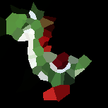
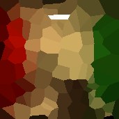
My approach is quite slow, but I'm very happy with quality of the results that it gives, particularly with respect to preserving edges. For example, here's Yoshi and the Cornell Box with just 1000 sites each:

There are two main parts that make it tick. The first, embodied in the evaluate() function takes a set of candidate site locations, sets the optimal colors on them and returns a score for the PSNR of the rendered Voronoi tessellation versus the target image. The colors for each site are determined by averaging target image pixels covered by the cell around the site. I use Welford's algorithm to help compute both the best color for each cell and the resulting PSNR using just a single pass over the image by exploiting the relationship between variance, MSE, and PSNR. This reduces the problem to one of finding the best set of site locations without particular regard to color.

The second part then, embodied in main(), tries to find this set. It starts by choosing a set of points at random. Then, in each step it removes one point (going round-robin) and tests a set of random candidate points to replace it. The one that yields the highest PSNR of the bunch is accepted and kept. Effectively, this causes the site to jump to a new location and generally improves the image bit-by-bit. Note that the algorithm intentionally does not retain the original location as a candidate. Sometimes this means that the jump lowers the overall image quality. Allowing this to happen helps to avoid getting stuck in local maxima. It also gives a stopping criteria; the program terminates after going a certain number of steps without improving on the best set of sites found so far.

Note that this implementation is fairly basic and can easily take hours of CPU-core time, especially as the number of sites grows. It recomputes the complete Voronoi map for every candidate and brute force tests the distance to all sites for each pixel. Since each operation involves removing one point at a time and adding another, the actual changes to the image at each step are going to be fairly local. There are algorithms for efficiently incrementally updating a Voronoi diagram and I believe they'd give this algorithm a tremendous speedup. For this contest, however, I've chosen to keep things simple and brute-force.

Code

#include <cstdlib>
#include <cmath>
#include <string>
#include <vector>
#include <fstream>
#include <istream>
#include <ostream>
#include <iostream>
#include <algorithm>
#include <random>

static auto const decimation = 2;
static auto const candidates = 96;
static auto const termination = 200;

using namespace std;

struct rgb {float red, green, blue;};
struct img {int width, height; vector<rgb> pixels;};
struct site {float x, y; rgb color;};

img read(string const &name) {
    ifstream file{name, ios::in | ios::binary};
    auto result = img{0, 0, {}};
    if (file.get() != 'P' || file.get() != '6')
        return result;
    auto skip = [&](){
        while (file.peek() < '0' || '9' < file.peek())
            if (file.get() == '#')
                while (file.peek() != '\r' && file.peek() != '\n')
                    file.get();
    };
     auto maximum = 0;
     skip(); file >> result.width;
     skip(); file >> result.height;
     skip(); file >> maximum;
     file.get();
     for (auto pixel = 0; pixel < result.width * result.height; ++pixel) {
         auto red = file.get() * 1.0f / maximum;
         auto green = file.get() * 1.0f / maximum;
         auto blue = file.get() * 1.0f / maximum;
         result.pixels.emplace_back(rgb{red, green, blue});
     }
     return result;
 }

 float evaluate(img const &target, vector<site> &sites) {
     auto counts = vector<int>(sites.size());
     auto variance = vector<rgb>(sites.size());
     for (auto &site : sites)
         site.color = rgb{0.0f, 0.0f, 0.0f};
     for (auto y = 0; y < target.height; y += decimation)
         for (auto x = 0; x < target.width; x += decimation) {
             auto best = 0;
             auto closest = 1.0e30f;
             for (auto index = 0; index < sites.size(); ++index) {
                 float distance = ((x - sites[index].x) * (x - sites[index].x) +
                                   (y - sites[index].y) * (y - sites[index].y));
                 if (distance < closest) {
                     best = index;
                     closest = distance;
                 }
             }
             ++counts[best];
             auto &pixel = target.pixels[y * target.width + x];
             auto &color = sites[best].color;
             rgb delta = {pixel.red - color.red,
                          pixel.green - color.green,
                          pixel.blue - color.blue};
             color.red += delta.red / counts[best];
             color.green += delta.green / counts[best];
             color.blue += delta.blue / counts[best];
             variance[best].red += delta.red * (pixel.red - color.red);
             variance[best].green += delta.green * (pixel.green - color.green);
             variance[best].blue += delta.blue * (pixel.blue - color.blue);
         }
     auto error = 0.0f;
     auto count = 0;
     for (auto index = 0; index < sites.size(); ++index) {
         if (!counts[index]) {
             auto x = min(max(static_cast<int>(sites[index].x), 0), target.width - 1);
             auto y = min(max(static_cast<int>(sites[index].y), 0), target.height - 1);
             sites[index].color = target.pixels[y * target.width + x];
         }
         count += counts[index];
         error += variance[index].red + variance[index].green + variance[index].blue;
     }
     return 10.0f * log10f(count * 3 / error);
 }

 void write(string const &name, int const width, int const height, vector<site> const &sites) {
     ofstream file{name, ios::out};
     file << width << " " << height << endl;
     for (auto const &site : sites)
         file << site.x << " " << site.y << " "
              << site.color.red << " "<< site.color.green << " "<< site.color.blue << endl;
 }

 int main(int argc, char **argv) {
     auto rng = mt19937{random_device{}()};
     auto uniform = uniform_real_distribution<float>{0.0f, 1.0f};
     auto target = read(argv[1]);
     auto sites = vector<site>{};
     for (auto point = atoi(argv[2]); point; --point)
         sites.emplace_back(site{
             target.width * uniform(rng),
             target.height * uniform(rng)});
     auto greatest = 0.0f;
     auto remaining = termination;
     for (auto step = 0; remaining; ++step, --remaining) {
         auto best_candidate = sites;
         auto best_psnr = 0.0f;
         #pragma omp parallel for
         for (auto candidate = 0; candidate < candidates; ++candidate) {
             auto trial = sites;
             #pragma omp critical
             {
                 trial[step % sites.size()].x = target.width * (uniform(rng) * 1.2f - 0.1f);
                 trial[step % sites.size()].y = target.height * (uniform(rng) * 1.2f - 0.1f);
             }
             auto psnr = evaluate(target, trial);
             #pragma omp critical
             if (psnr > best_psnr) {
                 best_candidate = trial;
                 best_psnr = psnr;
             }
         }
         sites = best_candidate;
         if (best_psnr > greatest) {
             greatest = best_psnr;
             remaining = termination;
             write(argv[3], target.width, target.height, sites);
         }
         cout << "Step " << step << "/" << remaining
              << ", PSNR = " << best_psnr << endl;
     }
     return 0;
 }

Running

The program is self-contained and has no external dependencies beyond the standard library, but it does require images to be in the binary PPM format. I use ImageMagick to convert images to PPM, though GIMP and quite a few other programs can do it too.

To compile it, save the program as voronoi.cpp and then run:

g++ -std=c++11 -fopenmp -O3 -o voronoi voronoi.cpp

I expect it will probably work on Windows with recent versions of Visual Studio, though I haven't tried this. You'll want to make sure that you're compiling with C++11 or better and OpenMP enabled if you do. OpenMP is not strictly necessary, but it helps a lot in making the execution times more tolerable.

To run it, do something like:

./voronoi cornell.ppm 1000 cornell-1000.txt

The later file will be updated with the site data as it goes. The first line will have the width and height of the image, followed by lines of x, y, r, g, b values suitable for copying and pasting into the Javascript renderer in the problem description.

The three constants at the top of the program allow you to tune it for speed versus quality. The decimation factor coarsens the target image when evaluating a set of sites for color and PSNR. The higher it is, the faster the program will run. Setting it to 1 uses the full resolution image. The candidates constant controls how many candidates to test on each step. Higher gives a better chance of finding a good spot to jump to but makes the program slower. Finally, termination is how many steps the program can go without improving its output before it quits. Increasing it may give better results but make it take marginally longer.

Images

N = 100, 300, 1000, and 3000:

Boojum

Posted 10 years ago

Reputation: 1 301

1This should've won IMO - much better than mine. – orlp – 10 years ago

1@orlp -- Thanks! To be fair though, you posted yours much sooner and it runs much more quickly. Speed counts! – Boojum – 10 years ago

1Well, mine isn't really a voronoi map answer :) It's a really really good sampling algorithm, but turning sample points into voronoi sites is clearly not optimal. – orlp – 10 years ago

55

IDL, adaptive refinement

This method is inspired by Adaptive Mesh Refinement from astronomical simulations, and also Subdivision surface. This is the kind of task that IDL prides itself on, which you'll be able to tell by the large number of builtin functions I was able to use. :D

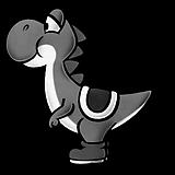
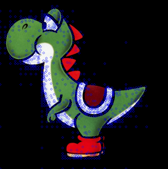
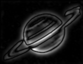
I've output some of the intermediates for the black-background yoshi test image, with n = 1000.

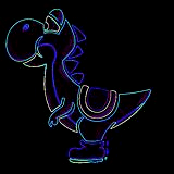
First, we perform a luminance greyscale on the image (using ct_luminance), and apply a Prewitt filter (prewitt, see wikipedia) for good edge detection:

abc abc

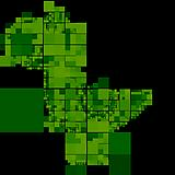
Then comes the real grunt-work: we subdivide the image into 4, and measure the variance in each quadrant in the filtered image. Our variance is weighted by the size of the subdivision (which in this first step is equal), so that "edgy" regions with high variance don't get subdivided smaller and smaller and smaller. Then, we use the weighted variance to target subdivisions with more detail, and iteratively subdivide each detail-rich section into 4 additional, until we hit our target number of sites (each subdivision contains exactly one site). Since we're adding 3 sites each time we iterate, we end up with n - 2 <= N <= n sites.

I made a .webm of the subdivision process for this image, which I can't embed, but it's here; the color in each subsection is determined by the weighted variance. (I made the same kind of video for the white-background yoshi, for comparison, with the color table reversed so it goes toward white instead of black; it's here.) The final product of the subdivision looks like this:

abc

Once we have our list of subdivisions, we go through each subdivision. The final site location is the position of the minimum of the Prewitt image, i.e., the least "edgy" pixel, and the color of the section is the color of that pixel; here's the original image, with sites marked:

abc

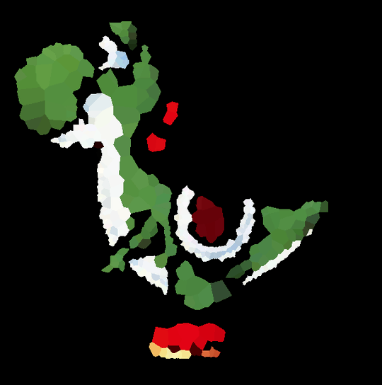
Then, we use the built-in triangulate to calculate the Delaunay triangulation of the sites, and the built-in voronoi to define the vertices of each Voronoi polygon, before drawing each polygon to an image buffer in its respective color. Finally, we save a snapshot of the image buffer.

abc

The code:

function subdivide, image, bounds, vars
  ;subdivide a section into 4, and return the 4 subdivisions and the variance of each
  division = list()
  vars = list()
  nx = bounds[2] - bounds[0]
  ny = bounds[3] - bounds[1]
  for i=0,1 do begin
    for j=0,1 do begin
      x = i * nx/2 + bounds[0]
      y = j * ny/2 + bounds[1]
      sub = image[x:x+nx/2-(~(nx mod 2)),y:y+ny/2-(~(ny mod 2))]
      division.add, [x,y,x+nx/2-(~(nx mod 2)),y+ny/2-(~(ny mod 2))]
      vars.add, variance(sub) * n_elements(sub)
    endfor
  endfor
  return, division
end

pro voro_map, n, image, outfile
  sz = size(image, /dim)
  ;first, convert image to greyscale, and then use a Prewitt filter to pick out edges
  edges = prewitt(reform(ct_luminance(image[0,*,*], image[1,*,*], image[2,*,*])))
  ;next, iteratively subdivide the image into sections, using variance to pick
  ;the next subdivision target (variance -> detail) until we've hit N subdivisions
  subdivisions = subdivide(edges, [0,0,sz[1],sz[2]], variances)
  while subdivisions.count() lt (n - 2) do begin
    !null = max(variances.toarray(),target)
    oldsub = subdivisions.remove(target)
    newsub = subdivide(edges, oldsub, vars)
    if subdivisions.count(newsub[0]) gt 0 or subdivisions.count(newsub[1]) gt 0 or subdivisions.count(newsub[2]) gt 0 or subdivisions.count(newsub[3]) gt 0 then stop
    subdivisions += newsub
    variances.remove, target
    variances += vars
  endwhile
  ;now we find the minimum edge value of each subdivision (we want to pick representative 
  ;colors, not edge colors) and use that as the site (with associated color)
  sites = fltarr(2,n)
  colors = lonarr(n)
  foreach sub, subdivisions, i do begin
    slice = edges[sub[0]:sub[2],sub[1]:sub[3]]
    !null = min(slice,target)
    sxy = array_indices(slice, target) + sub[0:1]
    sites[*,i] = sxy
    colors[i] = cgcolor24(image[0:2,sxy[0],sxy[1]])
  endforeach
  ;finally, generate the voronoi map
  old = !d.NAME
  set_plot, 'Z'
  device, set_resolution=sz[1:2], decomposed=1, set_pixel_depth=24
  triangulate, sites[0,*], sites[1,*], tr, connectivity=C
  for i=0,n-1 do begin
    if C[i] eq C[i+1] then continue
    voronoi, sites[0,*], sites[1,*], i, C, xp, yp
    cgpolygon, xp, yp, color=colors[i], /fill, /device
  endfor
  !null = cgsnapshot(file=outfile, /nodialog)
  set_plot, old
end

pro wrapper
  cd, '~/voronoi'
  fs = file_search()
  foreach f,fs do begin
    base = strsplit(f,'.',/extract)
    if base[1] eq 'png' then im = read_png(f) else read_jpeg, f, im
    voro_map,100, im, base[0]+'100.png'
    voro_map,500, im, base[0]+'500.png'
    voro_map,1000,im, base[0]+'1000.png'
  endforeach
end

Call this via voro_map, n, image, output_filename. I included a wrapper procedure as well, which went through each test image and ran with 100, 500, and 1000 sites.

Output collected here, and here are some thumbnails:

n = 100

abc abc abc abc abc abc abc abc abc abc abc abc abc

n = 500

abc abc abc abc abc abc abc abc abc abc abc abc abc

n = 1000

abc abc abc abc abc abc abc abc abc abc abc abc abc

sirpercival

Posted 10 years ago

Reputation: 1 824

9I really like the fact that this solution puts more points in more complex areas, which is I think the intent, and sets it apart from the others at this point. – alexander-brett – 10 years ago

yeah, the idea of detail-grouped points is what led me to adaptive refinement – sirpercival – 10 years ago

3Very neat explanation, and the images are impressive! I have a question--It looks like you get much different images when Yoshi is on a white background, where we have a few odd shapes. What might be causing that? – BrainSteel – 10 years ago

2@BrianSteel I imagine the outlines get picked up as high-variance areas and focused on unnecessarily, and then other truly high-detail areas have less points assigned because of that. – doppelgreener – 10 years ago

@BrainSteel i think doppel is right - there's a strong edge between the black border and the white background, which asks for a lot of detail in the algorithm. i'm not sure if this is something i can (or, more importantly, should) fix... – sirpercival – 10 years ago

47

Python 3 + PIL + SciPy, Fuzzy k-means

from collections import defaultdict
import itertools
import random
import time

from PIL import Image
import numpy as np
from scipy.spatial import KDTree, Delaunay

INFILE = "planet.jpg"
OUTFILE = "voronoi.txt"
N = 3000

DEBUG = True # Outputs extra images to see what's happening
FEATURE_FILE = "features.png"
SAMPLE_FILE = "samples.png"
SAMPLE_POINTS = 20000
ITERATIONS = 10
CLOSE_COLOR_THRESHOLD = 15

"""
Color conversion functions
"""

start_time = time.time()

# http://www.easyrgb.com/?X=MATH
def rgb2xyz(rgb):
  r, g, b = rgb
  r /= 255
  g /= 255
  b /= 255

  r = ((r + 0.055)/1.055)**2.4 if r > 0.04045 else r/12.92
  g = ((g + 0.055)/1.055)**2.4 if g > 0.04045 else g/12.92
  b = ((b + 0.055)/1.055)**2.4 if b > 0.04045 else b/12.92

  r *= 100
  g *= 100
  b *= 100

  x = r*0.4124 + g*0.3576 + b*0.1805
  y = r*0.2126 + g*0.7152 + b*0.0722
  z = r*0.0193 + g*0.1192 + b*0.9505

  return (x, y, z)

def xyz2lab(xyz):
  x, y, z = xyz
  x /= 95.047
  y /= 100
  z /= 108.883

  x = x**(1/3) if x > 0.008856 else 7.787*x + 16/116
  y = y**(1/3) if y > 0.008856 else 7.787*y + 16/116
  z = z**(1/3) if z > 0.008856 else 7.787*z + 16/116

  L = 116*y - 16
  a = 500*(x - y)
  b = 200*(y - z)

  return (L, a, b)

def rgb2lab(rgb):
  return xyz2lab(rgb2xyz(rgb))

def lab2xyz(lab):
  L, a, b = lab
  y = (L + 16)/116
  x = a/500 + y
  z = y - b/200

  y = y**3 if y**3 > 0.008856 else (y - 16/116)/7.787
  x = x**3 if x**3 > 0.008856 else (x - 16/116)/7.787
  z = z**3 if z**3 > 0.008856 else (z - 16/116)/7.787

  x *= 95.047
  y *= 100
  z *= 108.883

  return (x, y, z)

def xyz2rgb(xyz):
  x, y, z = xyz
  x /= 100
  y /= 100
  z /= 100

  r = x* 3.2406 + y*-1.5372 + z*-0.4986
  g = x*-0.9689 + y* 1.8758 + z* 0.0415
  b = x* 0.0557 + y*-0.2040 + z* 1.0570

  r = 1.055 * (r**(1/2.4)) - 0.055 if r > 0.0031308 else 12.92*r
  g = 1.055 * (g**(1/2.4)) - 0.055 if g > 0.0031308 else 12.92*g
  b = 1.055 * (b**(1/2.4)) - 0.055 if b > 0.0031308 else 12.92*b

  r *= 255
  g *= 255
  b *= 255

  return (r, g, b)

def lab2rgb(lab):
  return xyz2rgb(lab2xyz(lab))

"""
Step 1: Read image and convert to CIELAB
"""

im = Image.open(INFILE)
im = im.convert("RGB")
width, height = prev_size = im.size

pixlab_map = {}

for x in range(width):
    for y in range(height):
        pixlab_map[(x, y)] = rgb2lab(im.getpixel((x, y)))

print("Step 1: Image read and converted")

"""
Step 2: Get feature points
"""

def euclidean(point1, point2):
    return sum((x-y)**2 for x,y in zip(point1, point2))**.5


def neighbours(pixel):
    x, y = pixel
    results = []

    for dx, dy in itertools.product([-1, 0, 1], repeat=2):
        neighbour = (pixel[0] + dx, pixel[1] + dy)

        if (neighbour != pixel and 0 <= neighbour[0] < width
            and 0 <= neighbour[1] < height):
            results.append(neighbour)

    return results

def mse(colors, base):
    return sum(euclidean(x, base)**2 for x in colors)/len(colors)

features = []

for x in range(width):
    for y in range(height):
        pixel = (x, y)
        col = pixlab_map[pixel]
        features.append((mse([pixlab_map[n] for n in neighbours(pixel)], col),
                         random.random(),
                         pixel))

features.sort()
features_copy = [x[2] for x in features]

if DEBUG:
    test_im = Image.new("RGB", im.size)

    for i in range(len(features)):
        pixel = features[i][1]
        test_im.putpixel(pixel, (int(255*i/len(features)),)*3)

    test_im.save(FEATURE_FILE)

print("Step 2a: Edge detection-ish complete")

def random_index(list_):
    r = random.expovariate(2)

    while r > 1:
         r = random.expovariate(2)

    return int((1 - r) * len(list_))

sample_points = set()

while features and len(sample_points) < SAMPLE_POINTS:
    index = random_index(features)
    point = features[index][2]
    sample_points.add(point)
    del features[index]

print("Step 2b: {} feature samples generated".format(len(sample_points)))

if DEBUG:
    test_im = Image.new("RGB", im.size)

    for pixel in sample_points:
        test_im.putpixel(pixel, (255, 255, 255))

    test_im.save(SAMPLE_FILE)

"""
Step 3: Fuzzy k-means
"""

def euclidean(point1, point2):
    return sum((x-y)**2 for x,y in zip(point1, point2))**.5

def get_centroid(points):
    return tuple(sum(coord)/len(points) for coord in zip(*points))

def mean_cell_color(cell):
    return get_centroid([pixlab_map[pixel] for pixel in cell])

def median_cell_color(cell):
    # Pick start point out of mean and up to 10 pixels in cell
    mean_col = get_centroid([pixlab_map[pixel] for pixel in cell])
    start_choices = [pixlab_map[pixel] for pixel in cell]

    if len(start_choices) > 10:
        start_choices = random.sample(start_choices, 10)

    start_choices.append(mean_col)

    best_dist = None
    col = None

    for c in start_choices:
        dist = sum(euclidean(c, pixlab_map[pixel])
                       for pixel in cell)

        if col is None or dist < best_dist:
            col = c
            best_dist = dist

    # Approximate median by hill climbing
    last = None

    while last is None or euclidean(col, last) < 1e-6:
        last = col

        best_dist = None
        best_col = None

        for deviation in itertools.product([-1, 0, 1], repeat=3):
            new_col = tuple(x+y for x,y in zip(col, deviation))
            dist = sum(euclidean(new_col, pixlab_map[pixel])
                       for pixel in cell)

            if best_dist is None or dist < best_dist:
                best_col = new_col

        col = best_col

    return col

def random_point():
    index = random_index(features_copy)
    point = features_copy[index]

    dx = random.random() * 10 - 5
    dy = random.random() * 10 - 5

    return (point[0] + dx, point[1] + dy)

centroids = np.asarray([random_point() for _ in range(N)])
variance = {i:float("inf") for i in range(N)}
cluster_colors = {i:(0, 0, 0) for i in range(N)}

# Initial iteration
tree = KDTree(centroids)
clusters = defaultdict(set)

for point in sample_points:
    nearest = tree.query(point)[1]
    clusters[nearest].add(point)

# Cluster!
for iter_num in range(ITERATIONS):
    if DEBUG:
        test_im = Image.new("RGB", im.size)

        for n, pixels in clusters.items():
            color = 0xFFFFFF * (n/N)
            color = (int(color//256//256%256), int(color//256%256), int(color%256))

            for p in pixels:
                test_im.putpixel(p, color)

        test_im.save(SAMPLE_FILE)

    for cluster_num in clusters:
        if clusters[cluster_num]:
            cols = [pixlab_map[x] for x in clusters[cluster_num]]

            cluster_colors[cluster_num] = mean_cell_color(clusters[cluster_num])
            variance[cluster_num] = mse(cols, cluster_colors[cluster_num])

        else:
            cluster_colors[cluster_num] = (0, 0, 0)
            variance[cluster_num] = float("inf")

    print("Clustering (iteration {})".format(iter_num))

    # Remove useless/high variance
    if iter_num < ITERATIONS - 1:
        delaunay = Delaunay(np.asarray(centroids))
        neighbours = defaultdict(set)

        for simplex in delaunay.simplices:
            n1, n2, n3 = simplex

            neighbours[n1] |= {n2, n3}
            neighbours[n2] |= {n1, n3}
            neighbours[n3] |= {n1, n2}

        for num, centroid in enumerate(centroids):
            col = cluster_colors[num]

            like_neighbours = True

            nns = set() # neighbours + neighbours of neighbours

            for n in neighbours[num]:
                nns |= {n} | neighbours[n] - {num}

            nn_far = sum(euclidean(col, cluster_colors[nn]) > CLOSE_COLOR_THRESHOLD
                         for nn in nns)

            if nns and nn_far / len(nns) < 1/5:
                sample_points -= clusters[num]

                for _ in clusters[num]:
                    if features and len(sample_points) < SAMPLE_POINTS:
                        index = random_index(features)
                        point = features[index][3]
                        sample_points.add(point)
                        del features[index]

                clusters[num] = set()

    new_centroids = []

    for i in range(N):
        if clusters[i]:
            new_centroids.append(get_centroid(clusters[i]))
        else:
            new_centroids.append(random_point())

    centroids = np.asarray(new_centroids)
    tree = KDTree(centroids)

    clusters = defaultdict(set)

    for point in sample_points:
        nearest = tree.query(point, k=6)[1]
        col = pixlab_map[point]

        for n in nearest:
            if n < N and euclidean(col, cluster_colors[n])**2 <= variance[n]:
                clusters[n].add(point)
                break

        else:
            clusters[nearest[0]].add(point)

print("Step 3: Fuzzy k-means complete")

"""
Step 4: Output
"""

for i in range(N):
    if clusters[i]:
        centroids[i] = get_centroid(clusters[i])

centroids = np.asarray(centroids)
tree = KDTree(centroids)
color_clusters = defaultdict(set)

# Throw back on some sample points to get the colors right
all_points = [(x, y) for x in range(width) for y in range(height)]

for pixel in random.sample(all_points, int(min(width*height, 5 * SAMPLE_POINTS))):
    nearest = tree.query(pixel)[1]
    color_clusters[nearest].add(pixel)

with open(OUTFILE, "w") as outfile:
    for i in range(N):
        if clusters[i]:
            centroid = tuple(centroids[i])          
            col = tuple(x/255 for x in lab2rgb(median_cell_color(color_clusters[i] or clusters[i])))
            print(" ".join(map(str, centroid + col)), file=outfile)

print("Done! Time taken:", time.time() - start_time)

The algorithm

The core idea is that k-means clustering naturally partitions the image into Voronoi cells, since points are tied to the nearest centroid. However, we need to somehow add in the colours as a constraint.

First we convert each pixel to the Lab color space, for better colour manipulation.

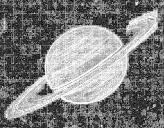
Then we do a sort of "poor man's edge detection". For each pixel, we look at its orthogonal and diagonal neighbours, and calculate the mean-squared difference in colour. We then sort all of the pixels by this difference, with pixels most similar to their neighbours at the front of the list, and pixels most dissimilar to their neighbours at the back (i.e., more likely to be an edge point). Here's an example for the planet, where the brighter the pixel is, the more different it is from its neighbours:

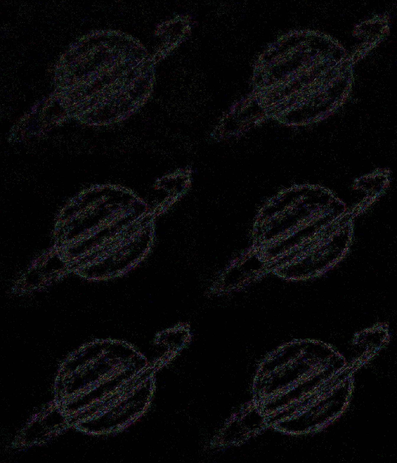
enter image description here

(There's a clear grid-like pattern on the rendered output above. According to @randomra, this is probably due to lossy JPG encoding, or imgur compressing the images.)

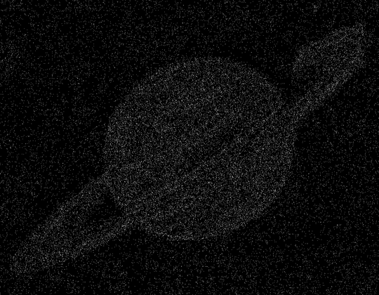
Next, we use this pixel ordering to sample a large number of points to be clustered. We use an exponential distribution, giving priority to points which are more edge-like and "interesting".

enter image description here

For the clustering, we first pick N centroids, randomly chosen using the same exponential distribution as above. An initial iteration is performed, and for each of the resulting clusters we assign a mean colour and a colour variance threshold. Then for a number of iterations, we:

  • Build the Delaunay triangulation of the centroids, so that we can easily query neighbours to centroids.
  • Use the triangulation to remove centroids which are close in colour to most (> 4/5) of their neighbours and neighbour's neighbours combined. Any associated sample points are also removed, and new replacement centroids and sample points are added. This step tries to force the algorithm to place more clusters where detail is needed.
  • Construct a kd-tree for the new centroids, so that we can easily query the closest centroids to any sample point.
  • Use the tree to assign each sample point to one of the 6 closest centroids (6 chosen empirically). A centroid will only accept a sample point if the point's colour is within the centroid's colour variance threshold. We try to assign each sample point to the first accepting centroid, but if that's not possible then we simply assign it to the closest centroid. The "fuzziness" of the algorithm comes from this step, since it's possible for clusters to overlap.
  • Recompute the centroids.

enter image description here

(Click for full size)

Finally, we sample a large number of points, this time using a uniform distribution. Using another kd-tree, we assign each point to its closest centroid, forming clusters. We then approximate the median colour of each cluster using a hill-climbing algorithm, giving our final cell colours (idea for this step thanks to @PhiNotPi and @MartinBüttner).

enter image description here

Notes

In addition to outputting a text file for the snippet (OUTFILE), if DEBUG is set to True the program will also output and overwrite the images above. The algorithm takes a couple of minutes for each image, so it's a good way of checking on progress which doesn't add an awful lot to the running time.

Sample outputs

N = 32:

enter image description here

N = 100:

enter image description here enter image description here enter image description here enter image description here enter image description here enter image description here enter image description here enter image description here enter image description here enter image description here enter image description here enter image description here enter image description here

N = 1000:

enter image description here enter image description here enter image description here enter image description here enter image description here enter image description here enter image description here enter image description here enter image description here enter image description here enter image description here enter image description here enter image description here

N = 3000:

enter image description here enter image description here enter image description here enter image description here enter image description here enter image description here enter image description here enter image description here enter image description here enter image description here enter image description here enter image description here enter image description here

Sp3000

Posted 10 years ago

Reputation: 58 729

1I really like how well your on-white Yoshis turned out. – Max – 10 years ago

26

Mathematica, Random Cells

This is the baseline solution, so you get an idea of the minimum I'm asking from you. Given the file name (locally or as a URL) in file and N in n, the following code simply picks out N random pixels, and uses the colours found at those pixels. This is really naive and doesn't work incredibly well, but I want you guys to beat this after all. :)

data = ImageData@Import@file;
dims = Dimensions[data][[1 ;; 2]]
{Reverse@#, data[[##]][[1 ;; 3]] & @@ Floor[1 + #]} &[dims #] & /@ 
 RandomReal[1, {n, 2}]

Here are all the test images for N = 100 (all images link to larger versions):

enter image description here enter image description here enter image description here enter image description here enter image description here enter image description here enter image description here enter image description here enter image description here enter image description here enter image description here enter image description here

As you can see, these are essentially useless. While they may have some artistic value, in an expressionist way, the original images are barely recognisable.

For N = 500, the situation is improved a bit, but there are still very odd artefacts, the images look washed out, and a lot of cells are wasted on regions without detail:

enter image description here enter image description here enter image description here enter image description here enter image description here enter image description here enter image description here enter image description here enter image description here enter image description here enter image description here enter image description here

Your turn!

Martin Ender

Posted 10 years ago

Reputation: 184 808

I'm not a good coder but my god these images are beautiful looking. Awesome idea! – Faraz Masroor – 10 years ago

Any reason for Dimensions@ImageData and not ImageDimensions? You can avoid the slow ImageData altogether by using PixelValue. – 2012rcampion – 10 years ago

@2012rcampion No reason, I just didn't know either function existed. I might fix that up later and also change the example images to the recommended N-values. – Martin Ender – 10 years ago

23

Mathematica

We all know Martin loves Mathematica so let me give it a try with Mathematica.

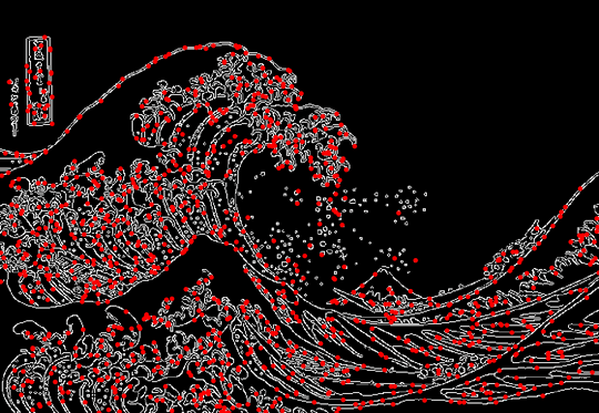
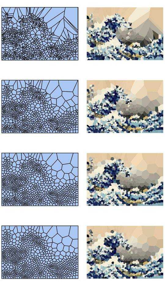
My algorithm uses random points from the image edges to create an initial voronoi diagram. The diagram is then prettified by an iterative adjustment of the mesh with a simple mean filter. This gives images with high cell density near high contrast regions and visually pleasing cells without crazy angles.

The following images show an example of the process in action. The fun is somewhat spoiled by Mathematicas bad Antialiasing, but we get vector graphics, that must be worth something.

This algorithm, without the random sampling, can be found in the VoronoiMesh documentation here.

enter image description here enter image description here

Test Images (100,300,1000,3000)

Code

VoronoiImage[img_, nSeeds_, iterations_] := Module[{
    i = img,
    edges = EdgeDetect@img,
    voronoiRegion = Transpose[{{0, 0}, ImageDimensions[img]}],
    seeds, voronoiInitial, voronoiRelaxed
    },
   seeds = RandomChoice[ImageValuePositions[edges, White], nSeeds];
   voronoiInitial = VoronoiMesh[seeds, voronoiRegion];
   voronoiRelaxed = 
    Nest[VoronoiMesh[Mean @@@ MeshPrimitives[#, 2], voronoiRegion] &, 
     voronoiInitial, iterations];
   Graphics[Table[{RGBColor[ImageValue[img, Mean @@ mp]], mp}, 
     {mp,MeshPrimitives[voronoiRelaxed, 2]}]]
   ];

paw

Posted 10 years ago

Reputation: 331

Nice job for a first post! :) You might want to try the Voronoi test image with 32 cells (that's the number of cells in the image itself). – Martin Ender – 10 years ago

Thanks! I guess my algorithm will perform terribly on this example. The seeds will get initialized on the cell edges and the recursion won't make it much better ;) – paw – 10 years ago

Despite slower rate to converge to the original image, I find that your algorithm yield a very artistry result! (like an improve version of Georges Seurat works). Great job! – neizod – 10 years ago

You can also get glassy looking interpolated polygon colours by changing your final lines to Graphics@Table[ Append[mp, VertexColors -> RGBColor /@ ImageValue[img, First[mp]]], {mp, MeshPrimitives[voronoiRelaxed, 2]}] – Histograms – 10 years ago

13

Python + SciPy + emcee

The algorithm I've used is the following:

  1. Resize images to a smallish size (~150 pixels)
  2. Make an unsharp-masked image of the maximum channel values (this helps not pick up white regions too strongly).
  3. Take the absolute value.
  4. Choose random points with a probability proportional to this image. This chooses points either side of discontinuities.
  5. Refine the chosen points to lower a cost function. The function is the maximum of the sum of the squared deviations in the channels (again helping bias to solid colours and not only solid white). I've misused Markov Chain Monte Carlo with the emcee module (highly recommended) as an optimiser. The procedure bails out when no new improvement is found after N chain iterations.

The algorithm appears to work very well. Unfortunately it can only sensibly run on smallish images. I haven't had time to take the Voronoi points and apply them to the larger images. They could be refined at this point. I could have also run the MCMC for longer to get better minima. The algorithm's weak point is that it is rather expensive. I haven't had time to increase beyond 1000 points and a couple of the 1000 point images are actually still being refined.

(right click and view image to get a bigger version)

Thumbnails for 100, 300 and 1000 points

Links to bigger versions are http://imgur.com/a/2IXDT#9 (100 points), http://imgur.com/a/bBQ7q (300 points) and http://imgur.com/a/rr8wJ (1000 points)

#!/usr/bin/env python

import glob
import os

import scipy.misc
import scipy.spatial
import scipy.signal
import numpy as N
import numpy.random as NR
import emcee

def compute_image(pars, rimg, gimg, bimg):
    npts = len(pars) // 2
    x = pars[:npts]
    y = pars[npts:npts*2]
    yw, xw = rimg.shape

    # exit if points are too far away from image, to stop MCMC
    # wandering off
    if(N.any(x > 1.2*xw) or N.any(x < -0.2*xw) or
       N.any(y > 1.2*yw) or N.any(y < -0.2*yw)):
        return None

    # compute tesselation
    xy = N.column_stack( (x, y) )
    tree = scipy.spatial.cKDTree(xy)

    ypts, xpts = N.indices((yw, xw))
    queryxy = N.column_stack((N.ravel(xpts), N.ravel(ypts)))

    dist, idx = tree.query(queryxy)

    idx = idx.reshape(yw, xw)
    ridx = N.ravel(idx)

    # tesselate image
    div = 1./N.clip(N.bincount(ridx), 1, 1e99)
    rav = N.bincount(ridx, weights=N.ravel(rimg)) * div
    gav = N.bincount(ridx, weights=N.ravel(gimg)) * div
    bav = N.bincount(ridx, weights=N.ravel(bimg)) * div

    rout = rav[idx]
    gout = gav[idx]
    bout = bav[idx]
    return rout, gout, bout

def compute_fit(pars, img_r, img_g, img_b):
    """Return fit statistic for parameters."""
    # get model
    retn = compute_image(pars, img_r, img_g, img_b)
    if retn is None:
        return -1e99
    model_r, model_g, model_b = retn

    # maximum squared deviation from one of the chanels
    fit = max( ((img_r-model_r)**2).sum(),
               ((img_g-model_g)**2).sum(),
               ((img_b-model_b)**2).sum() )

    # return fake log probability
    return -fit

def convgauss(img, sigma):
    """Convolve image with a Gaussian."""
    size = 3*sigma
    kern = N.fromfunction(
        lambda y, x: N.exp( -((x-size/2)**2+(y-size/2)**2)/2./sigma ),
        (size, size))
    kern /= kern.sum()
    out = scipy.signal.convolve2d(img.astype(N.float64), kern, mode='same')
    return out

def process_image(infilename, outroot, npts):
    img = scipy.misc.imread(infilename)
    img_r = img[:,:,0]
    img_g = img[:,:,1]
    img_b = img[:,:,2]

    # scale down size
    maxdim = max(img_r.shape)
    scale = int(maxdim / 150)
    img_r = img_r[::scale, ::scale]
    img_g = img_g[::scale, ::scale]
    img_b = img_b[::scale, ::scale]

    # make unsharp-masked image of input
    img_tot = N.max((img_r, img_g, img_b), axis=0)
    img1 = convgauss(img_tot, 2)
    img2 = convgauss(img_tot, 32)
    diff = N.abs(img1 - img2)
    diff = diff/diff.max()
    diffi = (diff*255).astype(N.int)
    scipy.misc.imsave(outroot + '_unsharp.png', diffi)

    # create random points with a probability distribution given by
    # the unsharp-masked image
    yw, xw = img_r.shape
    xpars = []
    ypars = []
    while len(xpars) < npts:
        ypar = NR.randint(int(yw*0.02),int(yw*0.98))
        xpar = NR.randint(int(xw*0.02),int(xw*0.98))
        if diff[ypar, xpar] > NR.rand():
            xpars.append(xpar)
            ypars.append(ypar)

    # initial parameters to model
    allpar = N.concatenate( (xpars, ypars) )

    # set up MCMC sampler with parameters close to each other
    nwalkers = npts*5  # needs to be at least 2*number of parameters+2
    pos0 = []
    for i in xrange(nwalkers):
        pos0.append(NR.normal(0,1,allpar.shape)+allpar)

    sampler = emcee.EnsembleSampler(
        nwalkers, len(allpar), compute_fit,
        args=[img_r, img_g, img_b],
        threads=4)

    # sample until we don't find a better fit
    lastmax = -N.inf
    ct = 0
    ct_nobetter = 0
    for result in sampler.sample(pos0, iterations=10000, storechain=False):
        print ct
        pos, lnprob = result[:2]
        maxidx = N.argmax(lnprob)

        if lnprob[maxidx] > lastmax:
            # write image
            lastmax = lnprob[maxidx]
            mimg = compute_image(pos[maxidx], img_r, img_g, img_b)
            out = N.dstack(mimg).astype(N.int32)
            out = N.clip(out, 0, 255)
            scipy.misc.imsave(outroot + '_binned.png', out)

            # save parameters
            N.savetxt(outroot + '_param.dat', scale*pos[maxidx])

            ct_nobetter = 0
            print(lastmax)

        ct += 1
        ct_nobetter += 1
        if ct_nobetter == 60:
            break

def main():
    for npts in 100, 300, 1000:
        for infile in sorted(glob.glob(os.path.join('images', '*'))):
            print infile
            outroot = '%s/%s_%i' % (
                'outdir',
                os.path.splitext(os.path.basename(infile))[0], npts)

            # race condition!
            lock = outroot + '.lock'
            if os.path.exists(lock):
                continue
            with open(lock, 'w') as f:
                pass

            process_image(infile, outroot, npts)

if __name__ == '__main__':
    main()

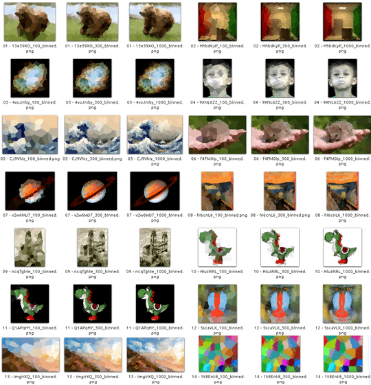
Unsharped-masked images look like the following. Random points are selected from the image if a random number is less than the value of the image (normed to 1):

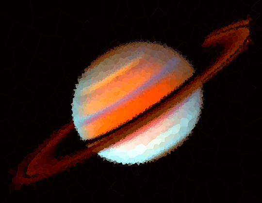
Unsharped masked Saturn image

I'll post bigger images and the Voronoi points if I get more time.

Edit: If you increase the number of walkers to 100*npts, change the cost function to be some of the squares of the deviations in all channels, and wait for a long time (increasing the number of iterations to break out of the loop to 200), it's possible to make some good images with just 100 points:

Image 11, 100 points Image 2, 100 points Image 4, 100 points Image 10, 100 points

xioxox

Posted 10 years ago

Reputation: 231

3

Using image energy as a point-weight map

In my approach to this challenge, I wanted a way to map "relevance" of a particular image area to the probability that a particular point would be chosen as a Voronoi centroid. However, I still wanted to preserve the artistic feel of Voronoi mosaicing by randomly choosing image points. Additionally, I wanted to operate on large images, so I don't lose anything in the downsampling process. My algorithm is roughly like this:

  1. For each image, create a sharpness map. The sharpness map is defined by the normalized image energy (or the square of the high frequency signal of the image). An example looks like this:

Sharpness map

  1. Generate a number of points from the image, taking 70 percent from the points in the sharpness map and 30 percent from all the other points. This means that points are sampled more densely from high-detail parts of the image.
  2. Color!

Results

N = 100, 500, 1000, 3000

Image 1, N = 100 Image 1, N = 500 Image 1, N = 1000 Image 1, N = 3000

Image 2, N = 100 Image 2, N = 500 Image 2, N = 1000 Image 2, N = 3000

Image 3, N = 100 Image 3, N = 500 Image 3, N = 1000 Image 3, N = 3000

Image 4, N = 100 Image 4, N = 500 Image 4, N = 1000 Image 4, N = 3000

Image 5, N = 100 Image 5, N = 500 Image 5, N = 1000 Image 5, N = 3000

Image 6, N = 100 Image 6, N = 500 Image 6, N = 1000 Image 6, N = 3000

Image 7, N = 100 Image 7, N = 500 Image 7, N = 1000 Image 7, N = 3000

Image 8, N = 100 Image 8, N = 500 Image 8, N = 1000 Image 8, N = 3000

Image 9, N = 100 Image 9, N = 500 Image 9, N = 1000 Image 9, N = 3000

Image 10, N = 100 Image 10, N = 500 Image 10, N = 1000 Image 10, N = 3000

Image 11, N = 100 Image 11, N = 500 Image 11, N = 1000 Image 11, N = 3000

Image 12, N = 100 Image 12, N = 500 Image 12, N = 1000 Image 12, N = 3000

Image 13, N = 100 Image 13, N = 500 Image 13, N = 1000 Image 13, N = 3000

Image 14, N = 100 Image 14, N = 500 Image 14, N = 1000 Image 14, N = 3000

mprat

Posted 10 years ago

Reputation: 155

14Would you mind a) including the source code used to generate this, and b) link each thumbnail to the full-size image? – Martin Ender – 10 years ago