PottersWheel
PottersWheel is a MATLAB toolbox for mathematical modeling of time-dependent dynamical systems that can be expressed as chemical reaction networks or ordinary differential equations (ODEs).[1] It allows the automatic calibration of model parameters by fitting the model to experimental measurements. CPU-intensive functions are written or – in case of model dependent functions – dynamically generated in C. Modeling can be done interactively using graphical user interfaces or based on MATLAB scripts using the PottersWheel function library. The software is intended to support the work of a mathematical modeler as a real potter's wheel eases the modeling of pottery.
| Developer(s) | TIKANIS GmbH, Freiburg, Germany |
|---|---|
| Initial release | October 6, 2006 |
| Stable release | 4.1.1
/ May 20, 2017 |
| Written in | MATLAB, C |
| Operating system | Microsoft Windows, Mac OS X, Linux |
| Size | 9 MB (250.000 lines) |
| Type | Mathematical modeling |
| License | Free trial license |
| Website | www.potterswheel.de |
Seven modeling phases
The basic use of PottersWheel covers seven phases from model creation to the prediction of new experiments.
Model creation

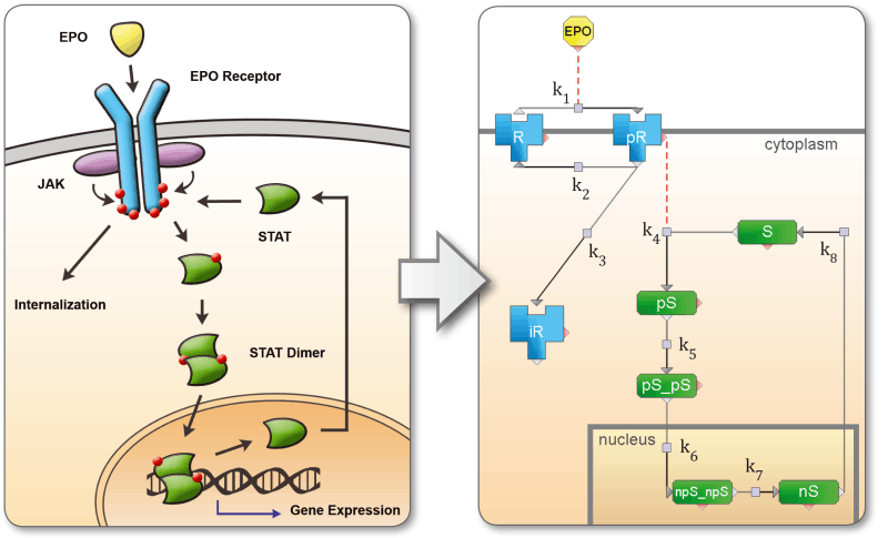
The dynamical system is formalized into a set of reactions or differential equations using a visual model designer or a text editor. The model is stored as a MATLAB *.m ASCII file. Modifications can therefore be tracked using a version control system like subversion or git. Model import and export is supported for SBML. Custom import-templates may be used to import custom model structures. Rule-based modeling is also supported, where a pattern represents a set of automatically generated reactions.
Example for a simple model definition file for a reaction network A → B → C → A with observed species A and C:
function m = getModel();

% Starting with an empty model
m = pwGetEmtptyModel();

% Adding reactions
m = pwAddR(m, 'A', 'B');
m = pwAddR(m, 'B', 'C');
m = pwAddR(m, 'C', 'A');

% Adding observables
m = pwAddY(m, 'A');
m = pwAddY(m, 'C');
Data import
External data saved in *.xls or *.txt files can be added to a model creating a model-data-couple. A mapping dialog allows to connect data column names to observed species names. Meta information in the data files comprise information about the experimental setting. Measurement errors are either stored in the data files, will be calculated using an error model, or are estimated automatically.
Parameter calibration
To fit a model to one or more data sets, the corresponding model-data-couples are combined into a fitting-assembly. Parameters like initial values, rate constants, and scaling factors can be fitted in an experiment-wise or global fashion. The user may select from several numerical integrators, optimization algorithms, and calibration strategies like fitting in normal or logarithmic parameter space.
Interpretation of the goodness-of-fit

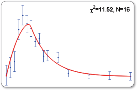
The quality of a fit is characterized by its chi-squared value. As a rule of thumb, for N fitted data points and p calibrated parameters, the chi-squared value should have a similar value as N − p or at least N. Statistically, this is expressed using a chi-squared test resulting in a p-value above a significance threshold of e.g. 0.05. For lower p-values, the model is
- either not able to explain the data and has to be refined,
- the standard deviation of the data points is actually larger than specified,
- or the used fitting strategy was not successful and the fit was trapped in a local minimum.
Apart from further chi-squared based characteristics like AIC and BIC, data-model-residual analyses exist, e.g. to investigate whether the residuals follow a Gaussian distribution. Finally, parameter confidence intervals may be estimated using either the Fisher information matrix approximation or based on the profile-likelihood function, if parameters are not unambiguously identifiable.
If the fit is not acceptable, the model has to be refined and the procedure continues with step 2. Else, the dynamic model properties can be examined and predictions calculated.
Model refinement
If the model structure is not able to explain the experimental measurements, a set of physiologically reasonable alternative models should be created. In order to avoid redundant model paragraphs and copy-and-paste errors, this can be done using a common core-model which is the same for all variants. Then, daughter-models are created and fitted to the data, preferably using batch processing strategies based on MATLAB scripts. As a starting point to envision suitable model variants, the PottersWheel equalizer may be used to understand the dynamic behavior of the original system.
Model analysis and prediction
A mathematical model may serve to display the concentration time-profile of unobserved species, to determine sensitive parameters representing potential targets within a clinical setting, or to calculate model characteristics like the half-life of a species.
Each analysis step may be stored into a modeling report, which may be exported as a Latex-based PDF.
Experimental design
An experimental setting corresponds to specific characteristics of driving input functions and initial concentrations. In a signal transduction pathway model the concentration of a ligand like EGF may be controlled experimentally. The driving input designer allows investigating the effect of a continuous, ramp, or pulse stimulation in combination with varying initial concentrations using the equalizer. In order to discriminate competing model hypotheses, the designed experiment should have as different observable time-profiles as possible.
Parameter identifiability
Many dynamical systems can only be observed partially, i.e. not all system species are accessible experimentally. For biological applications the amount and quality of experimental data is often limited. In this setting parameters can be structurally or practically non-identifiable. Then, parameters may compensate each other and fitted parameter values strongly depend on initial guesses. In PottersWheel non-identifiability can be detected using the Profile Likelihood Approach.[2] For characterizing functional relationships between the non-identifiable parameters PottersWheel applies random and systematic fit sequences.[3]
References
- T. Maiwald and J. Timmer (2008) "Dynamical Modeling and Multi-Experiment Fitting with PottersWheel", Bioinformatics 24(18):2037–2043
- Structural and practical identifiability analysis of partially observed dynamical models by exploiting the profile likelihood, A. Raue, C. Kreutz, T. Maiwald, J. Bachmann, M. Schilling, U. Klingmüller and J. Timmer, Bioinformatics 2009
- Data-based identifiability analysis of non-linear dynamical models, S. Hengl, C. Kreutz, J. Timmer and T. Maiwald, Bioinformatics 2007 23(19):2612–2618