Neural network Gaussian process

Bayesian networks are a modeling tool for assigning probabilities to events, and thereby characterizing the uncertainty in a model's predictions. Deep learning and artificial neural networks are approaches used in machine learning to build computational models which learn from training examples. Bayesian neural networks merge these fields. They are a type of artificial neural network whose parameters and predictions are both probabilistic.[1][2] While standard artificial neural networks often assign high confidence even to incorrect predictions,[3] Bayesian neural networks can more accurately evaluate how likely their predictions are to be correct.

Left: a Bayesian neural network with two hidden layers, transforming a 3-dimensional input (bottom) into a two-dimensional output ${\displaystyle (y_{1},y_{2})}$ (top). Right: output probability density function ${\displaystyle p(y_{1},y_{2})}$ induced by the random weights of the network. Video: as the width of the network increases, the output distribution simplifies, ultimately converging to a multivariate normal in the infinite width limit.

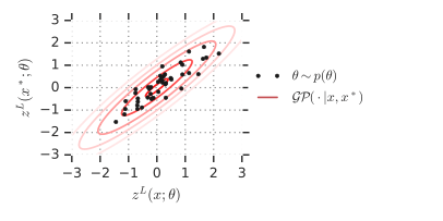
Neural Network Gaussian Processes (NNGPs) are equivalent to Bayesian neural networks in a particular limit,[4][5][6][7][8][9][10][11][12] and provide a closed form way to evaluate Bayesian neural networks. They are a Gaussian process probability distribution which describes the distribution over predictions made by the corresponding Bayesian neural network. Computation in artificial neural networks is usually organized into sequential layers of artificial neurons. The number of neurons in a layer is called the layer width. The equivalence between NNGPs and Bayesian neural networks occurs when the layers in a Bayesian neural network become infinitely wide (see figure). This large width limit is of practical interest, since finite width neural networks typically perform strictly better as layer width is increased.[13][14][8][15]

The NNGP also appears in several other contexts: it describes the distribution over predictions made by wide non-Bayesian artificial neural networks after random initialization of their parameters, but before training; it appears as a term in neural tangent kernel prediction equations; it is used in deep information propagation to characterize whether hyperparameters and architectures will be trainable.[16] It is related to other large width limits of neural networks.

A cartoon illustration

When parameters ${\displaystyle \theta }$ of an infinite width network are sampled repeatedly from their prior ${\displaystyle p(\theta )}$, the resulting distribution over network outputs is described by a Gaussian process.

Every setting of a neural network's parameters ${\displaystyle \theta }$ corresponds to a specific function computed by the neural network. A prior distribution ${\displaystyle p(\theta )}$ over neural network parameters therefore corresponds to a prior distribution over functions computed by the network. As neural networks are made infinitely wide, this distribution over functions converges to a Gaussian process for many architectures.

The figure to the right plots the one-dimensional outputs ${\displaystyle z^{L}(\cdot$ ;\theta )} of a neural network for two inputs ${\displaystyle x}$ and ${\displaystyle x^{*}}$ against each other. The black dots show the function computed by the neural network on these inputs for random draws of the parameters from ${\displaystyle p(\theta )}$. The red lines are iso-probability contours for the joint distribution over network outputs ${\displaystyle z^{L}(x;\theta )}$ and ${\displaystyle z^{L}(x^{*};\theta )}$ induced by ${\displaystyle p(\theta )}$. This is the distribution in function space corresponding to the distribution ${\displaystyle p(\theta )}$ in parameter space, and the black dots are samples from this distribution. For infinitely wide neural networks, since the distribution over functions computed by the neural network is a Gaussian process, the joint distribution over network outputs is a multivariate Gaussian for any finite set of network inputs.

The notation used in this section is the same as the notation used below to derive the correspondence between NNGPs and fully connected networks, and more details can be found there.

Architectures which correspond to an NNGP

The equivalence between infinitely wide Bayesian neural networks and NNGPs has been shown to hold for: single hidden layer[4] and deep[6][7] fully connected networks as the number of units per layer is taken to infinity; convolutional neural networks as the number of channels is taken to infinity;[8][9][10] transformer networks as the number of attention heads is taken to infinity;[17] recurrent networks as the number of units is taken to infinity[12]. In fact, this NNGP correspondence holds for almost any architecture: Generally, if an architecture can be expressed solely via matrix multiplication and coordinatewise nonlinearities (i.e. a tensor program), then it has an infinite-width GP[12]. This in particular includes all feedforward or recurrent neural networks composed of multilayer perceptron, recurrent neural networks (e.g. LSTMs, GRUs), (nD or graph) convolution, pooling, skip connection, attention, batch normalization, and/or layer normalization.

Correspondence between an infinitely wide fully connected network and a Gaussian process

This section will expand on the correspondence between infinitely wide neural networks and Gaussian processes for the specific case of a fully connected architecture. It will provide a proof sketch outlining why the correspondence holds, and introduce the specific functional form of the NNGP for fully connected networks. The proof sketch will closely follow the approach in Novak, et al., 2018.[8]

Network architecture specification

An NNGP is derived which is equivalent to a Bayesian neural network with this fully connected architecture.

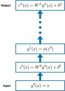
Consider a fully connected artificial neural network with inputs ${\displaystyle x}$, parameters ${\displaystyle \theta }$ consisting of weights ${\displaystyle W^{l}}$ and biases ${\displaystyle b^{l}}$ for each layer ${\displaystyle l}$ in the network, pre-activations (pre-nonlinearity) ${\displaystyle z^{l}}$, activations (post-nonlinearity) ${\displaystyle y^{l}}$, pointwise nonlinearity ${\displaystyle \phi (\cdot )}$, and layer widths ${\displaystyle n^{l}}$. For simplicity, the width ${\displaystyle n^{L+1}}$ of the readout vector ${\displaystyle z^{L}}$ is taken to be 1. The parameters of this network have a prior distribution ${\displaystyle p(\theta )}$, which consists of an isotropic Gaussian for each weight and bias, with the variance of the weights scaled inversely with layer width. This network is illustrated in the figure to the right, and described by the following set of equations:

${\displaystyle {\begin{aligned}x&\equiv {\text{input}}\\y^{l}(x)&=\left\{{\begin{array}{lcl}x&&l=0\\\phi \left(z^{l-1}(x)\right)&&l>0\end{array}}\right.\\z_{i}^{l}(x)&=\sum _{j}W_{ij}^{l}y_{j}^{l}(x)+b_{i}^{l}\\W_{ij}^{l}&\sim {\mathcal {N}}\left(0,{\frac {\sigma _{w}^{2}}{n^{l}}}\right)\\b_{i}^{l}&\sim {\mathcal {N}}\left(0,\sigma _{b}^{2}\right)\\\phi (\cdot )&\equiv {\text{nonlinearity}}\\y^{l}(x),z^{l-1}(x)&\in \mathbb {R} ^{n^{l}\times 1}\\n^{L+1}&=1\\\theta &=\left\{W^{0},b^{0},\dots ,W^{L},b^{L}\right\}\end{aligned}}}$

${\displaystyle z^{l}|y^{l}}$ is a Gaussian process

We first observe that the pre-activations ${\displaystyle z^{l}}$ are described by a Gaussian process conditioned on the preceding activations ${\displaystyle y^{l}}$. This result holds even at finite width. Each pre-activation ${\displaystyle z_{i}^{l}}$ is a weighted sum of Gaussian random variables, corresponding to the weights ${\displaystyle W_{ij}^{l}}$ and biases ${\displaystyle b_{i}^{l}}$, where the coefficients for each of those Gaussian variables are the preceding activations ${\displaystyle y_{j}^{l}}$. Because they are a weighted sum of zero-mean Gaussians, the ${\displaystyle z_{i}^{l}}$ are themselves zero-mean Gaussians (conditioned on the coefficients ${\displaystyle y_{j}^{l}}$). Since the ${\displaystyle z^{l}}$ are jointly Gaussian for any set of ${\displaystyle y^{l}}$, they are described by a Gaussian process conditioned on the preceding activations ${\displaystyle y^{l}}$. The covariance or kernel of this Gaussian process depends on the weight and bias variances ${\displaystyle \sigma _{w}^{2}}$ and ${\displaystyle \sigma _{b}^{2}}$, as well as the second moment matrix ${\displaystyle K^{l}}$ of the preceding activations ${\displaystyle y^{l}}$,

${\displaystyle {\begin{aligned}z_{i}^{l}\mid y^{l}&\sim {\mathcal {GP}}\left(0,\sigma _{w}^{2}K^{l}+\sigma _{b}^{2}\right)\\K^{l}(x,x')&={\frac {1}{n^{l}}}\sum _{i}y_{i}^{l}(x)y_{i}^{l}(x')\end{aligned}}}$

The effect of the weight scale ${\displaystyle \sigma _{w}^{2}}$ is to rescale the contribution to the covariance matrix from ${\displaystyle K^{l}}$, while the bias is shared for all inputs, and so ${\displaystyle \sigma _{b}^{2}}$ makes the ${\displaystyle z_{i}^{l}}$ for different datapoints more similar and makes the covariance matrix more like a constant matrix.

${\displaystyle z^{l}|K^{l}}$ is a Gaussian process

The pre-activations ${\displaystyle z^{l}}$ only depend on ${\displaystyle y^{l}}$ through its second moment matrix ${\displaystyle K^{l}}$. Because of this, we can say that ${\displaystyle z^{l}}$ is a Gaussian process conditioned on ${\displaystyle K^{l}}$, rather than conditioned on ${\displaystyle y^{l}}$,

${\displaystyle {\begin{aligned}z_{i}^{l}\mid K^{l}&\sim {\mathcal {GP}}\left(0,\sigma _{w}^{2}K^{l}+\sigma _{b}^{2}\right).\end{aligned}}}$

As layer width ${\displaystyle n^{l}\rightarrow \infty }$, ${\displaystyle K^{l}\mid K^{l-1}}$ becomes deterministic

As previously defined, ${\displaystyle K^{l}}$ is the second moment matrix of ${\displaystyle y^{l}}$. Since ${\displaystyle y^{l}}$ is the activation vector after applying the nonlinearity ${\displaystyle \phi }$, it can be replaced by ${\displaystyle \phi \left(z^{l-1}\right)}$, resulting in a modified equation expressing ${\displaystyle K^{l}}$ for ${\displaystyle l>0}$ in terms of ${\displaystyle z^{l-1}}$,

${\displaystyle {\begin{aligned}K^{l}(x,x')&={\frac {1}{n^{l}}}\sum _{i}\phi \left(z_{i}^{l-1}(x)\right)\phi \left(z_{i}^{l-1}(x')\right).\end{aligned}}}$

We have already determined that ${\displaystyle z^{l-1}|K^{l-1}}$ is a Gaussian process. This means that the sum defining ${\displaystyle K^{l}}$ is an average over ${\displaystyle n^{l}}$ samples from a Gaussian process which is a function of ${\displaystyle K^{l-1}}$,

${\displaystyle {\begin{aligned}\left\{z_{i}^{l-1}(x),z_{i}^{l-1}(x')\right\}&\sim {\mathcal {GP}}\left(0,\sigma _{w}^{2}K^{l-1}+\sigma _{b}^{2}\right).\end{aligned}}}$

As the layer width ${\displaystyle n^{l}}$ goes to infinity, this average over ${\displaystyle n^{l}}$ samples from the Gaussian process can be replaced with an integral over the Gaussian process:

${\displaystyle {\begin{aligned}\lim _{n^{l}\rightarrow \infty }K^{l}(x,x')&=\int dzdz'\phi (z)\phi (z'){\mathcal {N}}\left(\left[{\begin{array}{c}z\\z'\end{array}}\right];0,\sigma _{w}^{2}\left[{\begin{array}{cc}K^{l-1}(x,x)&K^{l-1}(x,x')\\K^{l-1}(x',x)&K^{l-1}(x',x')\end{array}}\right]+\sigma _{b}^{2}\right)\end{aligned}}}$

So, in the infinite width limit the second moment matrix ${\displaystyle K^{l}}$ for each pair of inputs ${\displaystyle x}$ and ${\displaystyle x'}$ can be expressed as an integral over a 2d Gaussian, of the product of ${\displaystyle \phi (z)}$ and ${\displaystyle \phi (z')}$. There are a number of situations where this has been solved analytically, such as when ${\displaystyle \phi (\cdot )}$ is a ReLU[18] or error function[5] nonlinearity. Even when it can't be solved analytically, since it is a 2d integral it can generally be efficiently computed numerically.[6] This integral is deterministic, so ${\displaystyle K^{l}|K^{l-1}}$ is deterministic.

For shorthand, we define a functional ${\displaystyle F}$, which corresponds to computing this 2d integral for all pairs of inputs, and which maps ${\displaystyle K^{l-1}}$ into ${\displaystyle K^{l}}$,

${\displaystyle {\begin{aligned}\lim _{n^{l}\rightarrow \infty }K^{l}&=F\left(K^{l-1}\right).\end{aligned}}}$

${\displaystyle z^{L}\mid x}$ is an NNGP

By recursively applying the observation that ${\displaystyle K^{l}\mid K^{l-1}}$ is deterministic as ${\displaystyle n^{l}\rightarrow \infty }$, ${\displaystyle K^{L}}$ can be written as a deterministic function of ${\displaystyle K^{0}}$,

${\displaystyle {\begin{aligned}\lim _{\min \left(n^{1},\dots ,n^{L}\right)\rightarrow \infty }K^{L}&=F\circ F\cdots \left(K^{0}\right)=F^{L}\left(K^{0}\right),\end{aligned}}}$

where ${\displaystyle F^{L}}$ indicates applying the functional ${\displaystyle F}$ sequentially ${\displaystyle L}$ times. By combining this expression with the further observations that the input layer second moment matrix ${\displaystyle K^{0}(x,x')={\frac {1}{n^{0}}}\sum _{i}x_{i}x'_{i}}$ is a deterministic function of the input ${\displaystyle x}$, and that ${\displaystyle z^{L}|K^{L}}$ is a Gaussian process, the output of the neural network can be expressed as a Gaussian process in terms of its input,

${\displaystyle {\begin{aligned}z_{i}^{L}(x)&\sim {\mathcal {GP}}\left(0,\sigma _{w}^{2}F^{L}\left(K^{0}\right)+\sigma _{b}^{2}\right).\end{aligned}}}$

Software libraries

Neural Tangents is a free and open-source Python library used for computing and doing inference with the NNGP and neural tangent kernel corresponding to various common ANN architectures.[19]

References

1. MacKay, David J. C. (1992). "A Practical Bayesian Framework for Backpropagation Networks". Neural Computation. 4 (3): 448–472. doi:10.1162/neco.1992.4.3.448. ISSN 0899-7667.
2. Neal, Radford M. (2012). Bayesian Learning for Neural Networks. Springer Science and Business Media.
3. Guo, Chuan; Pleiss, Geoff; Sun, Yu; Weinberger, Kilian Q. (2017). "On calibration of modern neural networks". Proceedings of the 34th International Conference on Machine Learning-Volume 70. arXiv:1706.04599.
4. Neal, Radford M. (1996), "Priors for Infinite Networks", Bayesian Learning for Neural Networks, Lecture Notes in Statistics, 118, Springer New York, pp. 29–53, doi:10.1007/978-1-4612-0745-0_2, ISBN 978-0-387-94724-2
5. Williams, Christopher K. I. (1997). "Computing with infinite networks". Neural Information Processing Systems.
6. Lee, Jaehoon; Bahri, Yasaman; Novak, Roman; Schoenholz, Samuel S.; Pennington, Jeffrey; Sohl-Dickstein, Jascha (2017). "Deep Neural Networks as Gaussian Processes". International Conference on Learning Representations. arXiv:1711.00165. Bibcode:2017arXiv171100165L.
7. G. de G. Matthews, Alexander; Rowland, Mark; Hron, Jiri; Turner, Richard E.; Ghahramani, Zoubin (2017). "Gaussian Process Behaviour in Wide Deep Neural Networks". International Conference on Learning Representations. arXiv:1804.11271. Bibcode:2018arXiv180411271M.
8. Novak, Roman; Xiao, Lechao; Lee, Jaehoon; Bahri, Yasaman; Yang, Greg; Abolafia, Dan; Pennington, Jeffrey; Sohl-Dickstein, Jascha (2018). "Bayesian Deep Convolutional Networks with Many Channels are Gaussian Processes". International Conference on Learning Representations. arXiv:1810.05148. Bibcode:2018arXiv181005148N.
9. Garriga-Alonso, Adrià; Aitchison, Laurence; Rasmussen, Carl Edward (2018). "Deep Convolutional Networks as shallow Gaussian Processes". International Conference on Learning Representations. arXiv:1808.05587. Bibcode:2018arXiv180805587G.
10. Borovykh, Anastasia (2018). "A Gaussian Process perspective on Convolutional Neural Networks". arXiv:1810.10798 [stat.ML].
11. Tsuchida, Russell; Pearce, Tim; van der Heide, Christopher; Roosta, Fred; Gallagher, Marcus (2020). "Avoiding Kernel Fixed Points: Computing with ELU and GELU Infinite Networks". arXiv:2002.08517 [cs.LG].
12. Yang, Greg (2019). "Tensor Programs I: Wide Feedforward or Recurrent Neural Networks of Any Architecture are Gaussian Processes" (PDF). Advances in Neural Information Processing Systems. arXiv:1910.12478. Bibcode:2019arXiv191012478Y.
13. Novak, Roman; Bahri, Yasaman; Abolafia, Daniel A.; Pennington, Jeffrey; Sohl-Dickstein, Jascha (2018-02-15). "Sensitivity and Generalization in Neural Networks: an Empirical Study". International Conference on Learning Representations. arXiv:1802.08760. Bibcode:2018arXiv180208760N.
14. Canziani, Alfredo; Paszke, Adam; Culurciello, Eugenio (2016-11-04). "An Analysis of Deep Neural Network Models for Practical Applications". arXiv:1605.07678. Bibcode:2016arXiv160507678C. Cite journal requires |journal= (help)
15. Neyshabur, Behnam; Li, Zhiyuan; Bhojanapalli, Srinadh; LeCun, Yann; Srebro, Nathan (2019). "Towards understanding the role of over-parametrization in generalization of neural networks". International Conference on Learning Representations. arXiv:1805.12076. Bibcode:2018arXiv180512076N.
16. Schoenholz, Samuel S.; Gilmer, Justin; Ganguli, Surya; Sohl-Dickstein, Jascha (2016). "Deep information propagation". International Conference on Learning Representations. arXiv:1611.01232.
17. Hron, Jiri; Bahri, Yasaman; Sohl-Dickstein, Jascha; Novak, Roman (2020-06-18). "Infinite attention: NNGP and NTK for deep attention networks". International Conference on Machine Learning. 2020. arXiv:2006.10540. Bibcode:2020arXiv200610540H.
18. Cho, Youngmin; Saul, Lawrence K. (2009). "Kernel Methods for Deep Learning". Neural Information Processing Systems: 342–350.
19. Novak, Roman; Xiao, Lechao; Hron, Jiri; Lee, Jaehoon; Alemi, Alexander A.; Sohl-Dickstein, Jascha; Schoenholz, Samuel S. (2019-12-05), "Neural Tangents: Fast and Easy Infinite Neural Networks in Python", International Conference on Learning Representations (ICLR), 2020, arXiv:1912.02803, Bibcode:2019arXiv191202803N