Local linearization method

In mathematics, specifically in numerical analysis, the Local Linearization (LL) method is a general strategy for designing numerical integrators for differential equations based on a local (piecewise) linearization of the given equation on consecutive time intervals. The numerical integrators are then iteratively defined as the solution of the resulting piecewise linear equation at the end of each consecutive interval. The LL method has been developed for a variety of equations such as the ordinary, delayed, random and stochastic differential equations. The LL integrators are key component in the implementation of inference methods for the estimation of unknown parameters and unobserved variables of differential equations given time series of (potentially noisy) observations. The LL schemes are ideals to deal with complex models in a variety of fields as neuroscience, finance, forestry management, control engineering, mathematical statistics, etc.

Background

Differential equations have become an important mathematical tool for describing the time evolution of several phenomenon, e.g., rotation of the planets around the sun, the dynamic of assets prices in the market, the fire of neurons, the propagation of epidemics, etc. However, since the exact solutions of these equations are usually unknown, numerical approximations to them obtained by numerical integrators are necessary. Currently, many applications in engineering and applied sciences focused in dynamical studies demand the developing of efficient numerical integrators that preserve, as much as possible, the dynamics of these equations. With this main motivation, the Local Linearization integrators have been developed.

High Order Local Linearization Method

High Order Local Linearization (HOLL) method is a generalization of the Local Linearization method oriented to obtain high order integrators for differential equations that preserve the stability and dynamics of the linear equations. The integrators are obtained by splitting, on consecutive time intervals, the solution x of the original equation in two parts: the solution z of the locally linearized equation plus a high order approximation of the residual ${\displaystyle \mathbf {r} =\mathbf {x} -\mathbf {z} }$.

Local Linearization scheme

A Local Linearization (LL) scheme is the final recursive algorithm that allows the numerical implementation of a discretization derived from the LL or HOLL method for a class of differential equations.

LL methods for ODEs

Consider the d-dimensional Ordinary Differential Equation (ODE)

${\displaystyle {\frac {d\mathbf {x} \left(t\right)}{dt}}=\mathbf {f} \left(t,\mathbf {x} \left(t\right)\right),\qquad t\in \left[t_{0},T\right],\qquad \qquad \qquad \qquad (4.1)}$

with initial condition ${\displaystyle \mathbf {x} (t_{0})=\mathbf {x} _{0}}$, where ${\displaystyle \mathbf {f} }$ is a differentiable function.

Let ${\displaystyle \left(t\right)_{h}=\{t_{n}:n=0,..,N\}}$ be a time discretization of the time interval ${\displaystyle [t_{0},T]}$ with maximum stepsize h such that ${\displaystyle t_{n}<t_{n+1}}$ and ${\displaystyle h_{n}=t_{n+1}-t_{n}\leq h}$. After the local linearization of the equation (1) at the time step ${\displaystyle t_{n}}$ the variation of constants formula yields

${\displaystyle \mathbf {x} (t_{n}+h)=\mathbf {x} (t_{n})+\mathbf {\phi } (t_{n},\mathbf {x} (t_{n});h)+\mathbf {r} (t_{n},\mathbf {x} (t_{n});h),}$

where

${\displaystyle \mathbf {\phi } (t_{n},\mathbf {z} _{n};h)=\int \limits _{0}^{h}e^{\mathbf {f} _{\mathbf {x} }\left(t_{n},\mathbf {z} _{n}\right)(h-s)}(\mathbf {f} \left(t_{n},\mathbf {z} _{n}\right)+\mathbf {f} _{t}\left(t_{n},\mathbf {z} _{n}\right)s)ds\qquad }$

results from the linear approximation, and

${\displaystyle \mathbf {r} (t_{n},\mathbf {z} _{n};h)=\int \limits _{0}^{h}e^{\mathbf {f} _{\mathbf {x} }\left(t_{n},\mathbf {z} _{n}\right)(h-s)}\mathbf {g} _{n}(s,\mathbf {x} (t_{n}+s))ds,\qquad \qquad \qquad (4.2)}$

is the residual of the linear approximation. Here, ${\displaystyle \mathbf {f} _{\mathbf {x} }}$ and ${\displaystyle \mathbf {f} _{t}}$ denote the partial derivatives of f with respect to the variables x and t, respectively, and ${\displaystyle \mathbf {g} _{n}(s,\mathbf {u} )=\mathbf {f} (s,\mathbf {u} )-\mathbf {f} _{\mathbf {x} }(t_{n},\mathbf {z} _{n})\mathbf {u} -\mathbf {f} _{t}\left(t_{n},\mathbf {z} _{n}\right)(s-t_{n})-\mathbf {f} \left(t_{n},\mathbf {z} _{n}\right)+\mathbf {f} _{\mathbf {x} }(t_{n},\mathbf {z} _{n})\mathbf {z} _{n}}$.

Local Linear discretization

For a time discretization ${\displaystyle \left(t\right)_{h}}$, the Local Linear discretization of the ODE (1) at each point ${\displaystyle t_{n+1}\in \left(t\right)_{h}}$ is defined by the recursive expression

${\displaystyle \mathbf {z} _{n+1}=\mathbf {z} _{n}+\mathbf {\phi } (t_{n},\mathbf {z} _{n};h_{n}),\qquad with\quad \mathbf {z} _{0}=\mathbf {x} _{0}{\text{.}}\qquad \qquad \qquad \qquad (4.3)}$

The Local Linear discretization (4.3) converges with order 2 to the solution of nonlinear ODEs, but it match the solution of the linear ODEs. The recursion (4.3) is also known as Exponential Euler discretization.

High Order Local Linear discretizations

For a time discretization ${\displaystyle \left(t\right)_{h},}$ a High Order Local Linear (HOLL) discretization of the ODE (1) at each point ${\displaystyle t_{n+1}\in \left(t\right)_{h}}$ is defined by the recursive expression

${\displaystyle \mathbf {z} _{n+1}=\mathbf {z} _{n}+\mathbf {\phi } (t_{n},\mathbf {z} _{n};h_{n})+{\widetilde {\mathbf {r} }}(t_{n},\mathbf {z} _{n};h_{n}),\qquad with\quad \mathbf {z} _{0}=\mathbf {x} _{0},\qquad \qquad \qquad (4.4)}$

where ${\displaystyle {\tilde {r}}}$ is an order ${\displaystyle \alpha }$ (>2) approximation to the residual r ${\displaystyle (i.e.,\left\vert \mathbf {r} (t_{n},\mathbf {z} _{n};h)-{\widetilde {\mathbf {r} }}(t_{n},\mathbf {z} _{n};h)\right\vert \propto h^{\alpha }).}$ The HOLL discretization (4.4) converges with order ${\displaystyle \alpha }$ to the solution of nonlinear ODEs, but it match the solution of the linear ODEs.

HOLL discretizations can be derived in two ways: 1) (quadrature-based) by approximating the integral representation (4.2) of r; and 2) (integrator-based) by using a numerical integrator for the differential representation of r defined by

${\displaystyle {\frac {d\mathbf {r} \left(t\right)}{dt}}=\mathbf {q} (t_{n},\mathbf {z} _{n};t\mathbf {,\mathbf {r} } \left(t\right)\mathbf {),} \qquad with\qquad \mathbf {r} \left(t_{n}\right)=\mathbf {0,} \qquad \qquad \qquad (4.5)}$

for all ${\displaystyle t\in \lbrack t_{k},t_{k+1}]}$, where

${\displaystyle \mathbf {q} (t_{n},\mathbf {z} _{n};s\mathbf {,\xi } )=\mathbf {f} (s,\mathbf {z} _{n}+\mathbf {\phi } \left(t_{n},\mathbf {z} _{n};s-t_{n}\right)+\mathbf {\xi } )-\mathbf {f} _{\mathbf {x} }(t_{n},\mathbf {z} _{n})\mathbf {\phi } \left(t_{n},\mathbf {z} _{n};s-t_{n}\right)-\mathbf {f} _{t}\left(t_{n},\mathbf {z} _{n}\right)(s-t_{n})-\mathbf {f} \left(t_{n},\mathbf {z} _{n}\right).}$

The quadrature-based discretization is often called Exponential Propagation Iterative or Exponential Rosenbrock, whereas the integrator-based one is called Locally Linearized discretization.

HOLL discretizations are, for instance, the followings:

• Locally Linearized Runge Kutta discretization

${\displaystyle \qquad \mathbf {z} _{n+1}=\mathbf {z} _{n}+\mathbf {\phi } (t_{n},\mathbf {z} _{n};h_{n})+h_{n}\sum _{j=1}^{s}b_{j}\mathbf {k} _{j},\quad with\quad \mathbf {k} _{i}=\mathbf {q} (t_{n},\mathbf {z} _{n};{\text{ }}t_{n}+c_{i}h_{n}\mathbf {,} \mathbf {} h_{n}\sum _{j=1}^{i-1}a_{ij}\mathbf {k} _{j}),}$

which is obtained by solving (4.5) via a s-stage Runge–Kutta (RK) scheme with coefficients ${\displaystyle \mathbf {c} =\left[c_{i}\right],\mathbf {A} =\left[a_{ij}\right]\quad and\quad \mathbf {b} =\left[b_{j}\right]}$.

• Local Linear Taylor discretization

$${\displaystyle \mathbf {z} _{n+1}=\mathbf {z} _{n}+\mathbf {\phi } (t_{n},\mathbf {z} _{n};h_{n})+\int _{0}^{h_{n}}e^{\left(h_{n}-s\right)\mathbf {f} _{\mathbf {x} }\left(t_{n},\mathbf {z} _{n}\right)}\sum _{j=2}^{p}{\frac {\mathbf {c} _{n,j}}{j!}}s^{j}ds,{\text{ with }}\mathbf {c} _{n,j}=\left({\frac {d^{j+1}\mathbf {x} \left(t\right)}{dt^{j+1}}}-\mathbf {f} _{\mathbf {x} }\left(t_{n},\mathbf {z} _{n}\right){\frac {d^{j}\mathbf {x} \left(t\right)}{dt^{j}}}\right)\mid _{t=\mathbf {z} _{n}},}$$

which results from the approximation of ${\displaystyle \mathbf {g} _{n}}$in (4.2) by its order-p truncated Taylor expansion.

• Multistep type Exponential Propagation discretization

${\textstyle \mathbf {z} _{n+1}=\mathbf {z} _{n}+\mathbf {\phi } (t_{n},\mathbf {z} _{n};h)+h\sum _{j=0}^{p-1}\gamma _{j}\nabla ^{j}\mathbf {g} _{n}(t_{n},\mathbf {z} _{n}),\quad with\quad \gamma _{j}=(-1)^{j}\int \limits _{0}^{1}e^{(1-\theta )h\mathbf {f} _{\mathbf {x} }\left(t_{n},\mathbf {z} _{n}\right)}\left({\begin{array}{c}-\theta \\j\end{array}}\right)d\theta ,}$

which results from the interpolation of ${\displaystyle \mathbf {g} _{n}}$in (4.2) by a polynomial of degree p on ${\displaystyle t_{n},\ldots ,t_{n-p+1}}$, where ${\displaystyle \nabla ^{j}\mathbf {g} _{n}(t_{m},\mathbf {z} _{m})}$ denotes the j-th backward difference of ${\displaystyle \mathbf {g} _{n}(t_{m},\mathbf {z} _{m})}$.

• Runge Kutta type Exponential Propagation discretization

${\textstyle \mathbf {z} _{n+1}=\mathbf {z} _{n}+\mathbf {\phi } (t_{n},\mathbf {z} _{n};h)+h\sum _{j=0}^{p-1}\gamma _{j,p}\nabla ^{j}\mathbf {g} _{n}(t_{n},\mathbf {z} _{n}),\quad with\quad \gamma _{j,p}=\int \limits _{0}^{1}e^{(1-\theta )h\mathbf {f} _{\mathbf {x} }\left(t_{n},\mathbf {z} _{n}\right)}\left({\begin{array}{c}\theta p\\j\end{array}}\right)d\theta ,}$

which results from the interpolation of ${\displaystyle \mathbf {g} _{n}}$in (4.2) by a polynomial of degree p on ${\displaystyle t_{n},\ldots ,t_{n}+(p-1)h/p}$,

• Linealized Exponential Adams discretization

${\textstyle \mathbf {z} _{n+1}=\mathbf {z} _{n}+\mathbf {\phi } (t_{n},\mathbf {z} _{n};h)+h\sum _{j=1}^{p-1}\sum _{l=1}^{j}{\frac {\gamma _{j+1}}{l}}\nabla ^{l}\mathbf {g} _{n}(t_{n},\mathbf {z} _{n}),\quad with\quad \gamma _{j+1}=(-1)^{j+1}\int \limits _{0}^{1}e^{(1-\theta )h\mathbf {f} _{\mathbf {x} }\left(t_{n},\mathbf {z} _{n}\right)}\theta \left({\begin{array}{c}-\theta \\j\end{array}}\right)d\theta ,}$

which results from the interpolation of ${\displaystyle \mathbf {g} _{n}}$in (4.2) by a Hermite polynomial of degree p on ${\displaystyle t_{n},\ldots ,t_{n-p+1}}$.

Local Linearization schemes

All numerical implementation ${\displaystyle \mathbf {y} _{n}}$ of the LL (or of a HOLL) discretization ${\displaystyle \mathbf {z} _{n}}$ involves approximations ${\displaystyle {\widetilde {\phi }}_{j}}$ to integrals ${\displaystyle \phi _{j}}$ of the form

${\displaystyle \phi _{j}(\mathbf {A} ,h)=\int \limits _{0}^{h}e^{(h-s)\mathbf {A} }s^{j-1}ds,\qquad j=1,2...,}$

where A is a d ${\displaystyle \times }$ d matrix. Every numerical implementation ${\displaystyle \mathbf {y} _{n}}$ of a Local Linear discretization ${\displaystyle \mathbf {z} _{n}}$ of any order is generically called Local Linearization scheme.

Computing integrals involving matrix exponential

Among a number of algorithms to compute the integrals ${\displaystyle \phi _{j}}$, those based on rational Padé and Krylov subspaces approximations for exponential matrix are preferred. For this, a central role is playing by the expression

${\displaystyle \sum \nolimits _{i=1}^{l}\phi _{i}(\mathbf {A} ,h)\mathbf {a} _{i}=\mathbf {L} e^{h\mathbf {H} }\mathbf {r,} }$

where ${\displaystyle \mathbf {a} _{i}}$ are d-dimensional vectors,

${\displaystyle \mathbf {H} ={\begin{bmatrix}\mathbf {A} &\mathbf {v} _{l}&\mathbf {v} _{l-1}&\cdots &\mathbf {v} _{1}\\\mathbf {0} &\mathbf {0} &1&\cdots &0\\\mathbf {0} &\mathbf {0} &0&\ddots &0\\\vdots &\vdots &\vdots &\ddots &1\\\mathbf {0} &\mathbf {0} &0&\cdots &0\end{bmatrix}}\in \mathbb {R} ^{(d+l)\times (d+l)},}$

${\displaystyle \mathbf {L} =[\mathbf {I} \quad \mathbf {0} _{d\times l}]}$, ${\displaystyle \mathbf {r} =[\mathbf {0} _{1\times (d+l-1)}\quad 1]^{\intercal }}$, ${\displaystyle \mathbf {v} _{i}=\mathbf {a} _{i}(i-1)!}$, being ${\displaystyle \mathbf {I} }$ the d-dimensional identity matrix.

If ${\displaystyle \mathbf {P} _{p,q}(2^{-k}\mathbf {H} h)}$ denotes the (p; q)-Padé approximation of ${\displaystyle e^{2^{-k}\mathbf {H} h}}$ and k is the smallest integer number such that ${\displaystyle |2^{-k}\mathbf {H} h|\leq {\frac {1}{2}},}$

${\displaystyle \left\vert \sum \nolimits _{i=1}^{l}\phi _{i}(\mathbf {A} ,h)\mathbf {a} _{i}-\mathbf {L} \left(\mathbf {\mathbf {P} } _{p,q}(2^{-k}\mathbf {H} h)\right)^{2^{k}}\mathbf {r} \right\vert \varpropto h^{p+q+1}.}$

If ${\displaystyle \mathbf {\mathbf {k} } _{m,k}^{p,q}(h,\mathbf {H} ,\mathbf {r} )}$ denotes the (m; p; q; k) Krylov-Padé approximation of ${\displaystyle e^{h\mathbf {H} }\mathbf {r} }$,

${\displaystyle \left\vert \sum \nolimits _{i=1}^{l}\phi _{i}(\mathbf {A} ,h)\mathbf {a} _{i}-\mathbf {L\mathbf {k} } _{m,k}^{p,q}(h,\mathbf {H} ,\mathbf {r} )\right\vert \varpropto h^{\min {m,p+q+1}},}$

where ${\displaystyle m\leq d}$ is the dimension of the Krylov subspace.

Order 2 LL schemes

${\displaystyle \mathbf {y} _{n+1}=\mathbf {y} _{n}+\mathbf {L} (\mathbf {P} _{p,q}(2^{-k_{n}}\mathbf {M} _{n}h_{n}))^{2^{k_{n}}}\mathbf {r,} \qquad \qquad (4.6)}$

where the matrices ${\displaystyle \mathbf {M} _{n}}$, L and r are defined as

${\displaystyle \mathbf {M} _{n}={\begin{bmatrix}\mathbf {f} _{\mathbf {x} }(t_{n},\mathbf {y} _{n})&\mathbf {f} _{t}(t_{n},\mathbf {y} _{n})&\mathbf {f} (t_{n},\mathbf {y} _{n})\\0&0&1\\0&0&0\end{bmatrix}}\in \mathbb {R} ^{(d+2)\times (d+2)},}$

${\displaystyle \mathbf {L} =\left[{\begin{array}{ll}\mathbf {I} &\mathbf {0} _{d\times 2}\end{array}}\right]}$ and ${\displaystyle \mathbf {r} ^{\intercal }=\left[{\begin{array}{ll}\mathbf {0} _{1\times (d+1)}&1\end{array}}\right]}$ with ${\displaystyle p+q>1}$ . For large systems of ODEs

${\displaystyle \mathbf {y} _{n+1}=\mathbf {y} _{n}+\mathbf {L\mathbf {k} } _{m_{n},k_{n}}^{p,q}(h_{n},\mathbf {M} _{n},\mathbf {r} )\mathbf {,} \qquad with\qquad m_{n}>1.}$

Order 3 LL-Taylor schemes

${\displaystyle \mathbf {y} _{n+1}=\mathbf {y} _{n}+\mathbf {L} _{1}(\mathbf {P} _{p,q}(2^{-k_{n}}\mathbf {T} _{n}h_{n}))^{2^{k_{n}}}\mathbf {r} _{1}\mathbf {,} \qquad \qquad (4.7)}$

where for autonomous ODEs the matrices ${\displaystyle \mathbf {T} _{n},\mathbf {L} _{1}}$ and ${\displaystyle \mathbf {r} _{1}}$ are defined as

${\displaystyle \mathbf {T} _{n}=\left[{\begin{array}{cccc}\mathbf {f} _{\mathbf {x} }(\mathbf {y} _{n})&(\mathbf {I} \otimes \mathbf {f} ^{\intercal }(\mathbf {y} _{n}))\mathbf {f} _{\mathbf {xx} }(\mathbf {y} _{n})\mathbf {f} (\mathbf {y} _{n})&\mathbf {0} &\mathbf {f} (\mathbf {y} _{n})\\0&0&0&0\\0&0&0&1\\0&0&0&0\end{array}}\right]\in \mathbb {R} ^{(d+3)\times (d+3)},}$

${\displaystyle \mathbf {L} _{1}=\left[{\begin{array}{ll}\mathbf {I} &\mathbf {0} _{d\times 3}\end{array}}\right]\quad and\quad \mathbf {r} _{1}^{\intercal }=\left[{\begin{array}{ll}\mathbf {0} _{1\times (d+2)}&1\end{array}}\right]}$. Here, ${\displaystyle \mathbf {f} _{\mathbf {xx} }}$ denotes the second derivative of f with respect to x, and p + q > 2. For large systems of ODEs

${\displaystyle \mathbf {y} _{n+1}=\mathbf {y} _{n}+\mathbf {L\mathbf {k} } _{m_{n},k_{n}}^{p,q}(h_{n},\mathbf {T} _{n},\mathbf {r} )\mathbf {,} \qquad with\qquad m_{n}>2.}$

Order 4 LL-RK schemes

${\displaystyle \mathbf {y} _{n+1}=\mathbf {y} _{n}+\mathbf {u} _{4}+{\frac {h_{n}}{6}}(2\mathbf {k} _{2}+2\mathbf {k} _{3}+\mathbf {k} _{4}),\qquad \qquad (4.8)}$

where

${\displaystyle \mathbf {u} _{j}=\mathbf {L} (\mathbf {P} _{p,q}(2^{-\kappa _{j}}\mathbf {M} _{n}c_{j}h_{n}))^{2^{\kappa _{j}}}\mathbf {r} }$

and

${\displaystyle \mathbf {k} _{j}=\mathbf {f} \left(t_{n}+c_{j}h_{n},\mathbf {y} _{n}+\mathbf {u} _{j}+c_{j}h_{n}\mathbf {k} _{j-1}\right)-\mathbf {f} \left(t_{n},\mathbf {y} _{n}\right)-\mathbf {f} _{\mathbf {x} }\left(t_{n},\mathbf {y} _{n}\right)\mathbf {u} _{j}\ -\mathbf {f} _{t}\left(t_{n},\mathbf {y} _{n}\right)c_{j}h_{n},}$

with ${\displaystyle \mathbf {k} _{1}\equiv \mathbf {0} ,c=\left[{\begin{array}{cccc}0&{\frac {1}{2}}&{\frac {1}{2}}&1\end{array}}\right],}$ and p + q > 3. For large systems of ODEs, the vector ${\displaystyle \mathbf {u} _{j}}$ in the above scheme is replaced by ${\displaystyle \mathbf {u} _{j}=\mathbf {L\mathbf {k} } _{m_{j},k_{j}}^{p,q}(c_{j}h_{n},\mathbf {M} _{n},\mathbf {r} ).}$

Locally Linearized Runge-Kutta of Dormand & Prince

${\displaystyle \mathbf {y} _{n+1}=\mathbf {y} _{n}+\mathbf {u} _{s}+h_{n}\sum _{j=1}^{s}b_{j}\mathbf {k} _{j}\qquad and\qquad {\widehat {\mathbf {y} }}_{n+1}=\mathbf {y} _{n}+\mathbf {u} _{s}+h_{n}\sum _{j=1}^{s}{\widehat {b}}_{j}\mathbf {k} _{j},\qquad \qquad (4.9)}$

where s = 6 is the number of stages,

${\displaystyle \mathbf {k} _{j}=\mathbf {f(} t_{n}+c_{j}h_{n},\mathbf {y} _{n}+\mathbf {u} _{j}+h_{n}\sum _{i=1}^{s-1}a_{j,i}\mathbf {k} _{i})-\mathbf {f} \left(t_{n},\mathbf {y} _{n}\right)-\mathbf {f} _{\mathbf {x} }\left(t_{n},\mathbf {y} _{n}\right)\mathbf {u} _{j}\ -\mathbf {f} _{t}\left(t_{n},\mathbf {y} _{n}\right)c_{j}h_{n},}$

with ${\displaystyle \mathbf {k} _{1}\equiv \mathbf {0} }$, and ${\displaystyle a_{j,i},b_{j},{\widehat {b}}_{j}\quad and\quad c_{j}}$ are the Runge-Kutta coefficients of Dormand and Prince and p + q > 4. For large systems of ODEs, the vector ${\displaystyle \mathbf {u} _{j}}$ in the above scheme is replaced by ${\displaystyle \mathbf {u} _{j}=\mathbf {L\mathbf {k} } _{m_{j},k_{j}}^{p,q}(c_{j}h_{n},\mathbf {M} _{n},\mathbf {r} ).}$

Stability and dynamics

Fig. 1 Phase portrait (dashed line) and approximate phase portrait (solid line) of the nonlinear ODE (4.10)-(4.11) computed by the LL2, RK4, LLRK4 schemes with step size h=1/2 , and p=q=6.

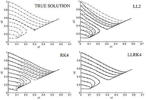
By construction, the LL and HOLL discretizations inherit the stability and dynamics of the linear ODEs, but it is not the case of the LL schemes in general. With ${\displaystyle p\leq q\leq p+2}$, the LL schemes (4.6)-(4.9) are A-stable. With q = p + 1 or q = p + 2, the LL schemes (4.6)-(4.9) are also L-stable. For linear ODEs, the LL schemes (4.6)-(4.9) converge with order p + q. In addition, with p = q = 6 and ${\displaystyle m_{n}}$ = d, all the above described LL schemes yield to the ″exact computation″ (up to the precision of the floating-point arithmetic) of linear ODEs on the current personal computers. This includes stiff and highly oscillatory linear equations. Moreover, the LL schemes (4.6)-(4.9) are regular for linear ODEs and inherit the symplectic structure of Hamiltonian harmonic oscillators. These LL schemes are also linearization preserving, and display a better reproduction of the stable and unstable manifolds around hyperbolic equilibrium points and periodic orbits that other numerical schemes with the same stepsize. For instance, Figure 1 shows the phase portrait of the ODEs

${\displaystyle {\frac {dx_{1}}{dt}}=-2x_{1}+x_{2}+1-\mu f\left(x_{1},\lambda \right)\qquad \qquad (4.10)}$ ${\displaystyle {\frac {dx_{2}}{dt}}=x_{1}-2x_{2}+1-\mu f\left(x_{2},\lambda \right)\qquad \qquad \quad (4.11)}$

with ${\displaystyle f\left(u,\lambda \right)=u\left(1+u+\lambda u^{2}\right)^{-1}}$, ${\displaystyle \mu =15}$ and ${\displaystyle \lambda =57}$, and its approximation by various schemes. This system has two stable stationary points and one unstable stationary point in the region ${\displaystyle 0\leq x_{1},x_{2}\leq 1}$.

LL methods for DDEs

Consider the d-dimensional Delay Differential Equation (DDE)

${\displaystyle {\frac {d\mathbf {x} \left(t\right)}{dt}}=\mathbf {f} \left(t,\mathbf {x} \left(t\right),\mathbf {x} _{t}(-\tau _{1}),\cdots ,\mathbf {x} _{t}(-\tau _{m})\right),\qquad t\in \left[t_{0},T\right],\qquad \qquad (5.1)}$

with m constant delays ${\displaystyle \tau _{i}>0}$ and initial condition ${\displaystyle \mathbf {x} _{t_{0}}(s)=\mathbf {\varphi } (s)}$ for all ${\displaystyle s\in \left[-\tau ,0\right],}$ where f is a differentiable function, ${\displaystyle \mathbf {x} _{t}:\left[-\tau ,0\right]\longrightarrow \mathbb {R} ^{d}}$ is the segment function defined as

${\displaystyle \mathbf {x} _{t}(s):=\mathbf {x} (t+s),{\text{ }}s\in \left[-\tau ,0\right],}$

for all ${\displaystyle t\in \left[t_{0},T\right],\mathbf {\varphi }$ :\left[-\tau ,0\right]\longrightarrow \mathbb {R} ^{d}} is a given function, and ${\displaystyle \tau =\max \left\{\tau _{1,}...,\tau _{m}\right\}.}$

Local Linear discretization

For a time discretization ${\displaystyle \left(t\right)_{h}}$ , the Local Linear discretization of the DDE (5.1) at each point ${\displaystyle t_{n+1}\in \left(t\right)_{h}}$ is defined by the recursive expression

${\displaystyle \mathbf {z} _{n+1}=\mathbf {z} _{n}+\Phi (t_{n},\mathbf {z} _{n},h_{n};{\widetilde {\mathbf {z} }}_{t_{n}}^{1},..,{\widetilde {\mathbf {z} }}_{t_{n}}^{m}),\qquad \qquad (5.2)}$

where

${\displaystyle \Phi (t_{n},\mathbf {z} _{n},h_{n};{\widetilde {\mathbf {z} }}_{t_{n}}^{1},..,{\widetilde {\mathbf {z} }}_{t_{n}}^{m})=\int \limits _{0}^{h_{n}}e^{\mathbf {A} _{n}(h_{n}-u)}[\sum \limits _{i=1}^{m}\mathbf {B} _{n}^{i}({\widetilde {\mathbf {z} }}_{t_{n}}^{i}\left(u-\tau _{i}\right)-{\widetilde {\mathbf {z} }}_{t_{n}}^{i}\left(-\tau _{i}\right))+\mathbf {d} _{n}]du+\int \limits _{0}^{h_{n}}\int \limits _{0}^{u}e^{\mathbf {A} _{n}(h_{n}-u)}\mathbf {c} _{n}drdu}$

${\displaystyle {\widetilde {\mathbf {z} }}_{t_{n}}^{i}:\left[-\tau _{i},0\right]\longrightarrow \mathbb {R} ^{d}}$ is the segment function defined as

${\displaystyle {\widetilde {\mathbf {z} }}_{t_{n}}^{i}(s):={\widetilde {\mathbf {z} }}^{i}(t_{n}+s),{\text{ }}s\in \left[-\tau _{i},0\right],}$

and ${\displaystyle {\widetilde {\mathbf {z} }}^{i}:\left[t_{n}-\tau _{i},t_{n}\right]\longrightarrow \mathbb {R} ^{d}}$is a suitable approximation to ${\displaystyle \mathbf {x} (t)}$ for all ${\displaystyle t\in \lbrack t_{n}-\tau _{i},t_{n}]}$ such that ${\displaystyle {\widetilde {\mathbf {z} }}^{i}(t_{n})=\mathbf {z} _{n}.}$ Here,

${\displaystyle \mathbf {A} _{n}=\mathbf {f} _{x}(t_{n},\mathbf {z} _{n},{\widetilde {\mathbf {z} }}_{t_{n}}^{1}(-\tau _{1}),...,{\widetilde {\mathbf {z} }}_{t_{n}}^{m}(-\tau _{d})),{\text{ }}\mathbf {B} _{n}^{i}=\mathbf {f} _{x_{t}(-\tau _{i})}(t_{n},\mathbf {z} _{n},{\widetilde {\mathbf {z} }}_{t_{n}}^{1}(-\tau _{1}),...,{\widetilde {\mathbf {z} }}_{t_{n}}^{m}(-\tau _{d}))}$

are constant matrices and

${\displaystyle \mathbf {c} _{n}=\mathbf {f} _{t}(t_{n},\mathbf {z} _{n},{\widetilde {\mathbf {z} }}_{t_{n}}^{1}(-\tau _{1}),...,{\widetilde {\mathbf {z} }}_{t_{n}}^{m}(-\tau _{d})){\text{ and }}\mathbf {d} _{n}=\mathbf {f(} t_{n},\mathbf {z} _{n},{\widetilde {\mathbf {z} }}_{t_{n}}^{1}(-\tau _{1}),...,{\widetilde {\mathbf {z} }}_{t_{n}}^{m}(-\tau _{d}))}$

are constant vectors. ${\displaystyle \mathbf {f} _{t},\mathbf {f} _{x}\quad and\quad \mathbf {f} _{x_{t}(-\tau _{i})}}$ denote, respectively, the partial derivatives of f with respect to the variables t and x, and ${\displaystyle \mathbf {x} _{t}(-\tau _{i})}$. The Local Linear discretization (5.2) converges to the solution of (5.1) with order ${\displaystyle \alpha =\min\{2,r\},}$ if ${\displaystyle {\widetilde {\mathbf {z} }}_{t_{n}}^{i}}$ approximates ${\displaystyle \mathbf {z} _{t_{n}}^{i}}$ with order ${\displaystyle r\quad (i.e.,\left\vert \mathbf {z} _{t_{n}}^{i}\mathbf {(} u-\tau _{i}\mathbf {)} -{\widetilde {\mathbf {z} }}_{t_{n}}^{i}\mathbf {(} u-\tau _{i}\mathbf {)} \right\vert \propto h_{n}^{r}}$ for all ${\displaystyle u\in \lbrack 0,h_{n}])}$.

Local Linearization schemes

Fig. 2 Approximate paths of the Marchuk et al. (1991) antiviral immune model described by a stiff system of ten-dimensional nonlinear DDEs with five time delays. Step-size h=0.01 fixed, and p=q=6.

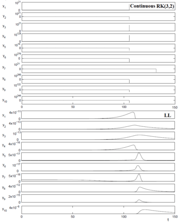
Depending of the approximations ${\displaystyle {\widetilde {\mathbf {z} }}_{t_{n}}^{i}}$ and of the algorithm to compute ${\displaystyle \mathbf {\phi } }$ different Local Linearizations schemes can be defined. Every numerical implementation ${\displaystyle \mathbf {y} _{n}}$ of a Local Linear discretization ${\displaystyle \mathbf {z} _{n}}$ is generically called Local Linearization scheme.

Order 2 Polynomial LL schemes

${\displaystyle \mathbf {y} _{n+1}=\mathbf {y} _{n}+\mathbf {L} (\mathbf {P} _{p,q}(2^{-k_{n}}\mathbf {M} _{n}h_{n}))^{2^{k_{n}}}\mathbf {r,} \qquad \qquad \qquad (5.3)}$

where the matrices ${\displaystyle \mathbf {M} _{n},\mathbf {L} }$ and ${\displaystyle \mathbf {r} }$ are defined as

${\displaystyle \mathbf {M} _{n}={\begin{bmatrix}\mathbf {A} _{n}&\mathbf {c} _{n}+\sum \limits _{i=1}^{m}\mathbf {B} _{n}^{i}\mathbf {\alpha } _{n}^{i}&\mathbf {d} _{n}\\0&0&1\\0&0&0\end{bmatrix}}\in \mathbb {R} ^{(d+2)\times (d+2)},}$

${\displaystyle \mathbf {L} =\left[{\begin{array}{ll}\mathbf {I} &\mathbf {0} _{d\times 2}\end{array}}\right]}$ and ${\displaystyle \mathbf {r} ^{\intercal }=\left[{\begin{array}{ll}\mathbf {0} _{1\times (d+1)}&1\end{array}}\right],h_{n}\leq \tau }$, and ${\displaystyle p+q>1}$. Here, the matrices ${\displaystyle \mathbf {A} _{n}}$, ${\displaystyle \mathbf {B} _{n}^{i}}$, ${\displaystyle \mathbf {c} _{n}}$ and ${\displaystyle \mathbf {d} _{n}}$ are defined as in (5.2), but replacing ${\displaystyle \mathbf {z} }$ by ${\displaystyle \mathbf {y} }$ and ${\displaystyle \mathbf {\alpha } _{n}^{i}=(\mathbf {y} (t_{n+1}-\tau _{i})-\mathbf {y} (t_{n}-\tau _{i}))/h_{n},}$ where

${\displaystyle \mathbf {y} \left(t\right)=\mathbf {y} _{n_{t}}+\mathbf {L} (\mathbf {P} _{p,q}(2^{-k_{n}}\mathbf {M} _{n_{t}}(t-t_{n_{t}})))^{2^{k_{n}}}\mathbf {r} ,}$

with ${\displaystyle n_{t}=\max\{n=0,1,2,...,:t_{n}\leq t{\text{ and }}t_{n}\in \left(t\right)_{h}\}}$, is the Local Linear Approximation to the solution of (5.1) defined through the LL scheme (5.3) for all ${\displaystyle t\in \lbrack t_{0},t_{n}]}$ and by ${\displaystyle \mathbf {y} \left(t\right)=\mathbf {\varphi } \left(t\right)}$ for ${\displaystyle t\in \left[t_{0}-\tau ,t_{0}\right]}$. For large systems of DDEs

${\displaystyle \mathbf {y} _{n+1}=\mathbf {y} _{n}+\mathbf {L\mathbf {k} } _{m_{n},k_{n}}^{p,q}(h_{n},\mathbf {M} _{n},\mathbf {r} )\quad and\quad \mathbf {y} \left(t\right)=\mathbf {y} _{n_{t}}+\mathbf {L\mathbf {k} } _{m_{n_{t}},k_{n_{t}}}^{p,q}(t-t_{n_{t}},\mathbf {M} _{n_{t}},\mathbf {r} ),}$

with ${\displaystyle p+q>1}$ and ${\displaystyle m_{n}>2}$.

LL methods for RDEs

Consider the d-dimensional Random Differential Equation (RDE)

${\displaystyle {\frac {d\mathbf {x} \left(t\right)}{dt}}=\mathbf {f} (\mathbf {x} (t),\mathbf {\xi } (t)),\quad t\in \left[t_{0},T\right],\qquad \qquad \qquad (6.1)}$

with initial condition ${\displaystyle \mathbf {x} (t_{0})=\mathbf {x} _{0},}$ where ${\displaystyle \mathbf {\xi } }$ is a k-dimensional separable finite continuous stochastic process, and f is a differentiable function. Suppose that a realization (path) of ${\displaystyle \mathbf {\xi } }$ is given.

Local Linear discretization

For a time discretization ${\displaystyle \left(t\right)_{h}}$, the Local Linear discretization of the RDE (6.1) at each point ${\displaystyle t_{n+1}\in \left(t\right)_{h}}$ is defined by the recursive expression

${\displaystyle \mathbf {z} _{n+1}=\mathbf {z} _{n}+\mathbf {\phi } (t_{n},\mathbf {z} _{n};h_{n}),\qquad with\qquad \mathbf {z} _{0}=\mathbf {x} _{0},}$

where

${\displaystyle \mathbf {\phi } (t_{n},\mathbf {z} _{n};h_{n})=\int \limits _{0}^{h_{n}}e^{\mathbf {f} _{\mathbf {x} }\left(\mathbf {z} _{n},\mathbf {\xi } (t_{n})\right)(h_{n}-u)}(\mathbf {f(z} _{n},\mathbf {\xi } (t_{n}))+\mathbf {f} _{\mathbf {\xi } }(\mathbf {z} _{n},\mathbf {\xi } (t_{n}))({\widetilde {\mathbf {\xi } }}(t_{n}+u)-{\widetilde {\mathbf {\xi } }}(t_{n})))du}$

and ${\displaystyle {\widetilde {\mathbf {\xi } }}}$ is an approximation to the process ${\displaystyle \mathbf {\xi } }$ for all ${\displaystyle t\in \left[t_{0},T\right].}$ Here, ${\displaystyle \mathbf {f} _{x}}$ and ${\displaystyle \mathbf {f} _{\xi }}$ denote the partial derivatives of ${\displaystyle \mathbf {f} }$ with respect to ${\displaystyle \mathbf {x} }$ and ${\displaystyle \xi }$, respectively.

Local Linearization schemes

Fig. 3 Phase portrait of trajectories of the Euler and LL schemes in the integration of the nonlinear RDE (6.2)-(6.3) with step size h=1/32, and p=q=6.

Depending of the approximations ${\displaystyle {\widetilde {\mathbf {\xi } }}}$ to the process ${\displaystyle \mathbf {\xi } }$ and of the algorithm to compute ${\displaystyle \mathbf {\phi } }$ different Local Linearizations schemes can be defined. Every numerical implementation ${\displaystyle \mathbf {y} _{n}}$ of the Local Linear discretization ${\displaystyle \mathbf {z} _{n}}$ is generically called Local Linearization scheme.

LL schemes

${\displaystyle \mathbf {y} _{n+1}=\mathbf {y} _{n}+\mathbf {L} (\mathbf {P} _{p,q}(2^{-k_{n}}\mathbf {M} _{n}h_{n}))^{2^{k_{n}}}\mathbf {r,} }$

where the matrices ${\displaystyle \mathbf {M} _{n},\quad \mathbf {L} \quad and\quad \mathbf {r} }$ are defined as

${\displaystyle \mathbf {M} _{n}=\left[{\begin{array}{ccc}\mathbf {f} _{\mathbf {x} }\left(\mathbf {y} _{n},\mathbf {\xi } (t_{n})\right)&\mathbf {f} _{\mathbf {\xi } }(\mathbf {y} _{n},\mathbf {\xi } (t_{n})(\mathbf {\xi } (t_{n+1})-\mathbf {\xi } (t_{n}))/h_{n}&\mathbf {f} \left(\mathbf {y} _{n},\mathbf {\xi } (t_{n})\right)\\0&0&1\\0&0&0\end{array}}\right]\in \mathbb {R} ^{(d+2)\times (d+2)},}$

${\displaystyle \mathbf {L} =\left[{\begin{array}{ll}\mathbf {I} &\mathbf {0} _{d\times 2}\end{array}}\right]}$, ${\displaystyle \mathbf {r} ^{\intercal }=\left[{\begin{array}{ll}\mathbf {0} _{1\times (d+1)}&1\end{array}}\right]}$, and p+q>1. For large systems of RDEs,

${\displaystyle \mathbf {y} _{n+1}=\mathbf {y} _{n}+\mathbf {L\mathbf {k} } _{m_{n},k_{n}}^{p,q}(h_{n},\mathbf {M} _{n},\mathbf {r} ),\quad p+q>1\quad and\quad m_{n}>2.}$

The convergence rate of both schemes is ${\displaystyle min\{2,2\gamma \}}$, where is ${\displaystyle \gamma }$ the exponent of the Holder condition of ${\displaystyle \mathbf {\xi } }$.

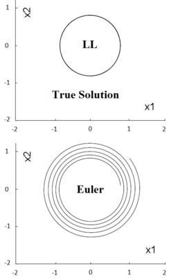
Figure 3 presents the phase portrait of the RDE

${\displaystyle {\frac {dx_{1}}{dt}}=-x_{2}+\left(1-x_{1}^{2}-x_{2}^{2}\right)x_{1}\sin(w^{H}(t))^{2},\qquad \qquad x_{1}(0)=0.8\qquad (6.2)}$

${\displaystyle {\frac {dx_{2}}{dt}}=x_{1}+(1-x_{1}^{2}-x_{2}^{2})x_{2}\sin(w^{H}(t))^{2},\qquad \qquad x_{2}(0)=0.1,\qquad (6.3)}$

and its approximation by two numerical schemes, where ${\displaystyle w^{H}}$ denotes a fractional Brownian process with Hurst exponent H=0.45.

Strong LL methods for SDEs

Consider the d-dimensional Stochastic Differential Equation (SDE)

${\displaystyle d\mathbf {x} (t)=\mathbf {f} (t,\mathbf {x} (t))dt+\sum \limits _{i=1}^{m}\mathbf {g} _{i}(t)d\mathbf {w} ^{i}(t),\quad t\in \left[t_{0},T\right],\qquad \qquad \qquad (7.1)}$

with initial condition ${\displaystyle \mathbf {x} (t_{0})=\mathbf {x} _{0}}$, where the drift coefficient ${\displaystyle \mathbf {f} }$ and the diffusion coefficient ${\displaystyle \mathbf {g} _{i}}$ are differentiable functions, and ${\displaystyle \mathbf {w=(\mathbf {w} } ^{1},\ldots ,\mathbf {w} ^{m}\mathbf {)} }$ is an m-dimensional standard Wiener process.

Local Linear discretization

For a time discretization ${\displaystyle \left(t\right)_{h}}$ , the order-${\displaystyle \mathbb {\gamma } }$ (=1,1.5) Strong Local Linear discretization of the solution of the SDE (7.1) is defined by the recursive relation

${\displaystyle \mathbf {z} _{n+1}=\mathbf {z} _{n}+\mathbf {\phi } _{\mathbb {\gamma } }(t_{n},\mathbf {z} _{n};h_{n})+\mathbf {\xi } (t_{n},\mathbf {z} _{n};h_{n}),\quad with\quad \mathbf {z} _{0}=\mathbf {x} _{0},}$

where

${\displaystyle \mathbf {\phi } _{\mathbb {\gamma } }(t_{n},\mathbf {z} _{n};\delta )=\int _{0}^{\delta }e^{\mathbf {f} _{\mathbf {x} }(t_{n},\mathbf {y} _{n})(\delta -u)}(\mathbf {f(} t_{n},\mathbf {z} _{n})+\mathbf {a} ^{\mathbb {\gamma } }(t_{n},\mathbf {z} _{n})u)du}$

and

${\displaystyle \mathbf {\xi } \left(t_{n},\mathbf {z} _{n};\delta \right)=\sum \limits _{i=1}^{m}\int \nolimits _{t_{n}}^{t_{n}+\delta }e^{\mathbf {f} _{\mathbf {x} }(t_{n},\mathbf {z} _{n})(t_{n}+\delta -u)}\mathbf {g} _{i}(u)d\mathbf {w} ^{i}(u).}$

Here,

${\displaystyle \mathbf {a} ^{\mathbb {\gamma } }(t_{n},\mathbf {z} _{n})=\left\{{\begin{matrix}\mathbf {f} _{t}(t_{n},\mathbf {z} _{n})&\qquad for\qquad \mathbb {\gamma } =1\\\mathbf {f} _{t}(t_{n},\mathbf {z} _{n})+{\frac {1}{2}}\sum \limits _{j=1}^{m}\left(\mathbf {I} \otimes \mathbf {g} _{j}^{\intercal }\left(t_{n}\right)\right)\mathbf {f} _{\mathbf {xx} }(t_{n},\mathbf {z} _{n})\mathbf {g} _{j}\left(t_{n}\right)&\quad for\quad \mathbb {\gamma } =1.5,\end{matrix}}\right.}$

${\displaystyle \mathbf {f} _{\mathbf {x} },\mathbf {f} _{t}}$ denote the partial derivatives of ${\displaystyle \mathbf {f} }$ with respect to the variables ${\displaystyle \mathbf {x} }$ and t, respectively, and ${\displaystyle \mathbf {f} _{\mathbf {xx} }}$ the Hessian matrix of ${\displaystyle \mathbf {f} }$ with respect to ${\displaystyle \mathbf {x} }$. The strong Local Linear discretization ${\displaystyle \mathbf {z} _{n+1}}$ converges with order ${\displaystyle \mathbb {\gamma } }$ (=1,1.5) to the solution of (7.1).

High Order Local Linear discretizations

After the local linearization of the drift term of (7.1) at ${\displaystyle (t_{n},\mathbf {z} _{n})}$, the equation for the residual ${\displaystyle \mathbf {r} }$ is given by

${\displaystyle d\mathbf {r} \left(t\right)=\mathbf {q} _{\gamma }(t_{n},\mathbf {z} _{n};t\mathbf {,\mathbf {r} } \left(t\right))dt+\sum \limits _{i=1}^{m}\mathbf {g} _{i}(t)d\mathbf {w} ^{i}(t)\mathbf {,} \qquad \mathbf {r} \left(t_{n}\right)=\mathbf {0} }$

for all ${\displaystyle t\in \lbrack t_{n},t_{n+1}]}$, where

${\displaystyle \mathbf {q} _{\gamma }(t_{n},\mathbf {z} _{n};s\mathbf {,\xi } )=\mathbf {f} (s,\mathbf {z} _{n}+\mathbf {\phi } _{\gamma }\left(t_{n},\mathbf {z} _{n};s-t_{n}\right)+\mathbf {\xi } )-\mathbf {f} _{\mathbf {x} }(t_{n},\mathbf {z} _{n})\mathbf {\phi } _{\gamma }\left(t_{n},\mathbf {z} _{n};s-t_{n}\right)-\mathbf {a} ^{\gamma }\left(t_{n},\mathbf {z} _{n}\right)(s-t_{n})-\mathbf {f} \left(t_{n},\mathbf {z} _{n}\right).}$

High Order Local Linear discretization of the SDE (7.1) at each point ${\displaystyle t_{n+1}\in \left(t\right)_{h}}$ is then defined by the recursive expression

${\displaystyle \mathbf {z} _{n+1}=\mathbf {z} _{n}+\mathbf {\phi } _{\gamma }(t_{n},\mathbf {z} _{n};h_{n})+{\widetilde {\mathbf {r} }}(t_{n},\mathbf {z} _{n};h_{n}),\qquad with\qquad \mathbf {z} _{0}=\mathbf {x} _{0},}$

where ${\displaystyle {\widetilde {\mathbf {r} }}}$ is a strong approximation to the residual ${\displaystyle \mathbf {r} }$ of order ${\displaystyle \alpha }$ higher than 1.5. The strong HOLL discretization ${\displaystyle \mathbf {z} _{n+1}}$ converges with order ${\displaystyle \alpha }$ to the solution of (7.1).

Local Linearization schemes

Depending on the way of computing ${\displaystyle \mathbf {\phi } _{\mathbb {\gamma } }}$ , ${\displaystyle \mathbf {\xi } }$ and ${\displaystyle {\widetilde {\mathbf {r} }}}$ different numerical schemes could be obtained. Every numerical implementation ${\displaystyle \mathbf {y} _{n}}$ of a strong Local Linear discretization ${\displaystyle \mathbf {z} _{n}}$ of any order is generically called Strong Local Linearization scheme.

Order 1 SLL schemes

${\displaystyle \mathbf {y} _{n+1}=\mathbf {y} _{n}+\mathbf {L} (\mathbf {P} _{p,q}(2^{-k_{n}}\mathbf {M} _{n}h_{n}))^{2^{k_{n}}}\mathbf {r+} \sum \limits _{i=1}^{m}\mathbf {g} _{i}(t_{n})\Delta \mathbf {w} _{n}^{i},\qquad \qquad (7.2)}$

where the matrices ${\displaystyle \mathbf {M} _{n}}$, ${\displaystyle \mathbf {L} }$ and ${\displaystyle \mathbf {r} }$ are defined as in (4.6), ${\displaystyle \Delta \mathbf {w} _{n}^{i}}$ is an i.i.d. zero mean Gaussian random variable with variance ${\displaystyle h_{n}}$, and p+q>1. For large systems of SDEs, in the above scheme ${\displaystyle (\mathbf {P} _{p,q}(2^{-k_{n}}\mathbf {M} _{n}h_{n}))^{2^{k_{n}}}\mathbf {r} }$ is replaced by ${\displaystyle \mathbf {\mathbf {k} } _{m_{n},k_{n}}^{p,q}(h_{n},\mathbf {M} _{n},\mathbf {r} )}$.

Order 1.5 SLL schemes

${\displaystyle \mathbf {y} _{n+1}=\mathbf {y} _{n}+\mathbf {L} (\mathbf {P} _{p,q}(2^{-k_{n}}\mathbf {M} _{n}h_{n}))^{2^{k_{n}}}\mathbf {r} +\sum \limits _{i=1}^{m}\left(\mathbf {g} _{i}(t_{n})\Delta \mathbf {w} _{n}^{i}+\mathbf {f} _{\mathbf {x} }(t_{n},{\widetilde {\mathbf {y} }}_{n})\mathbf {g} _{i}(t_{n})\Delta \mathbf {z} _{n}^{i}+{\frac {d\mathbf {g} _{i}(t_{n})}{dt}}(\Delta \mathbf {w} _{n}^{i}h_{n}-\Delta \mathbf {z} _{n}^{i})\right),\qquad \qquad (7.3)}$

where the matrices ${\displaystyle \mathbf {M} _{n}}$, ${\displaystyle \mathbf {L} }$ and ${\displaystyle \mathbf {r} }$ are defined as

${\displaystyle \mathbf {M} _{n}={\begin{bmatrix}\mathbf {f} _{\mathbf {x} }(t_{n},\mathbf {y} _{n})&\mathbf {f} _{t}(t_{n},\mathbf {y} _{n})+{\frac {1}{2}}\sum \limits _{j=1}^{m}\left(\mathbf {I} \otimes \mathbf {g} _{j}^{\intercal }\left(t_{n}\right)\right)\mathbf {f} _{\mathbf {xx} }(t_{n},\mathbf {y} _{n})\mathbf {g} _{j}\left(t_{n}\right)&\mathbf {f} (t_{n},\mathbf {y} _{n})\\0&0&1\\0&0&0\end{bmatrix}}\in \mathbb {R} ^{(d+2)\times (d+2)},}$

${\displaystyle \mathbf {L} =\left[{\begin{array}{ll}\mathbf {I} &\mathbf {0} _{d\times 2}\end{array}}\right],\mathbf {r} ^{\intercal }=\left[{\begin{array}{ll}\mathbf {0} _{1\times (d+1)}&1\end{array}}\right]}$, ${\displaystyle \Delta \mathbf {z} _{n}^{i}}$ is a i.i.d. zero mean Gaussian random variable with variance ${\displaystyle E\left((\Delta \mathbf {z} _{n}^{i})^{2}\right)={\frac {1}{3}}h_{n}^{3}}$ and covariance ${\displaystyle E(\Delta \mathbf {w} _{n}^{i}\Delta \mathbf {z} _{n}^{i})={\frac {1}{2}}h_{n}^{2}}$ and p+q>1. For large systems of SDEs, in the above scheme ${\displaystyle (\mathbf {P} _{p,q}(2^{-k_{n}}\mathbf {M} _{n}h_{n}))^{2^{k_{n}}}\mathbf {r} }$ is replaced by ${\displaystyle \mathbf {\mathbf {k} } _{m_{n},k_{n}}^{p,q}(h_{n},\mathbf {M} _{n},\mathbf {r} )}$.

Order 2 SLL-Taylor schemes

${\displaystyle \mathbf {y} _{t_{n+1}}=\mathbf {y} _{n}+\mathbf {L} (\mathbf {P} _{p,q}(2^{-k_{n}}\mathbf {M} _{n}h_{n}))^{2^{k_{n}}}\mathbf {r} +\sum \limits _{j=1}^{m}\mathbf {g} _{j}\left(t_{n}\right)\Delta \mathbf {w} _{n}^{j}+\sum \limits _{j=1}^{m}\mathbf {f} _{\mathbf {x} }(t_{n},\mathbf {y} _{n})\mathbf {g} _{j}\left(t_{n}\right){\widetilde {J}}_{\left(j,0\right)}+\sum \limits _{j=1}^{m}{\frac {d\mathbf {g} _{_{j}}}{dt}}\left(t_{n}\right){\widetilde {J}}_{\left(0,j\right)}}$

${\displaystyle \qquad \qquad +\sum \limits _{j_{1},j_{2}=1}^{m}\left(\mathbf {I} \otimes \mathbf {g} _{j_{2}}^{\intercal }\left(t_{n}\right)\right)\mathbf {f} _{\mathbf {xx} }(t_{n},\mathbf {y} _{n})\mathbf {g} _{j_{1}}\left(t_{n}\right){\widetilde {J}}_{\left(j_{1},j_{2},0\right)},\qquad \qquad \qquad (7.4)}$

where ${\displaystyle \mathbf {M} _{n}}$, ${\displaystyle \mathbf {L} }$, ${\displaystyle \mathbf {r} }$ and ${\displaystyle \Delta \mathbf {w} _{n}^{i}}$ are defined as in the order-1 SLL schemes, and ${\displaystyle {\widetilde {J}}_{\alpha }}$ is order 2 approximation to the multiple Stratonovish integral ${\displaystyle J_{\alpha }}$.

Order 2 SLL-RK schemes

Fig. 4, Top: Evolution of domains in the phase plane of the harmonic oscillator (7.6), with ε=0 and ω=σ=1. Images of the initial unit circle (green) are obtained at three time moments T by the exact solution (black), and by the schemes SLL1 (blue) and Implicit Euler (red) with h=0.05. Bottom: Expected value of the energy (solid line) along the solution of the nonlinear oscillator (7.6), with ε=1 and ω=100, and its approximation (circles) computed via Monte Carlo with 10000 simulations of the SLL1 scheme with h=1/2 and p=q=6.

For SDEs with a single Wiener noise (m=1)

${\displaystyle \mathbf {y} _{t_{n+1}}=\mathbf {y} _{n}+{\widetilde {\mathbf {\phi } }}(t_{n},\mathbf {y} _{n};h_{n})+{\frac {h_{n}}{2}}\left(\mathbf {k} _{1}+\mathbf {k} _{2}\right)+\mathbf {g} \left(t_{n}\right)\Delta w_{n}+{\frac {\left(\mathbf {g} \left(t_{n+1}\right)-\mathbf {g} \left(t_{n}\right)\right)}{h_{n}}}J_{\left(0,1\right)}\qquad \qquad (7.5)}$

where

${\displaystyle \mathbf {k} _{1}=\mathbf {f} (t_{n}+{\frac {h_{n}}{2}},\mathbf {y} _{n}+{\widetilde {\mathbf {\phi } }}(t_{n},\mathbf {y} _{n};{\frac {h_{n}}{2}})+\gamma _{+})-\mathbf {f} _{\mathbf {x} }(t_{n},\mathbf {y} _{n}){\widetilde {\mathbf {\phi } }}(t_{n},\mathbf {y} _{n};{\frac {h_{n}}{2}})-\mathbf {f} \left(t_{n},\mathbf {y} _{n}\right)-\mathbf {f} _{t}\left(t_{n},\mathbf {y} _{n}\right){\frac {h_{n}}{2}},}$${\displaystyle \mathbf {k} _{2}=\mathbf {f} (t_{n}+{\frac {h_{n}}{2}},\mathbf {y} _{n}+{\widetilde {\mathbf {\phi } }}(t_{n},\mathbf {y} _{n};{\frac {h_{n}}{2}})+\gamma _{-})-\mathbf {f} _{\mathbf {x} }(t_{n},\mathbf {y} _{n}){\widetilde {\mathbf {\phi } }}(t_{n},\mathbf {y} _{n};{\frac {h_{n}}{2}})-\mathbf {f} \left(t_{n},\mathbf {y} _{n}\right)-\mathbf {f} _{t}\left(t_{n},\mathbf {y} _{n}\right){\frac {h_{n}}{2}},}$

with ${\displaystyle \gamma _{\pm }={\frac {1}{h_{n}}}\mathbf {g} \left(t_{n}\right){\Bigl (}{\widetilde {J}}_{\left(1,0\right)}\pm {\sqrt {2{\widetilde {J}}_{\left(1,1,0\right)}h_{n}-{\widetilde {J}}_{\left(1,0\right)}^{2}}}{\Bigr )}}$. Here, ${\displaystyle {\widetilde {\mathbf {\phi } }}(t_{n},\mathbf {y} _{n};h_{n})=\mathbf {L} (\mathbf {P} _{p,q}(2^{-k_{n}}\mathbf {M} _{n}h_{n}))^{2^{k_{n}}}\mathbf {r} }$ for low dimensional SDEs, and ${\displaystyle {\widetilde {\mathbf {\phi } }}(t_{n},\mathbf {y} _{n};h_{n})=\mathbf {L\mathbf {k} } _{m_{n},k_{n}}^{p,q}(h_{n},\mathbf {M} _{n},\mathbf {r} )}$ for large systems of SDEs, where ${\displaystyle \mathbf {M} _{n}}$, ${\displaystyle \mathbf {L} }$, ${\displaystyle \mathbf {r} }$, ${\displaystyle \Delta \mathbf {w} _{n}^{i}}$ and ${\displaystyle {\widetilde {J}}_{\alpha }}$ are defined as in the order-2 SLL-Taylor schemes, p+q>1 and ${\displaystyle m_{n}>2}$.

Stability and dynamics

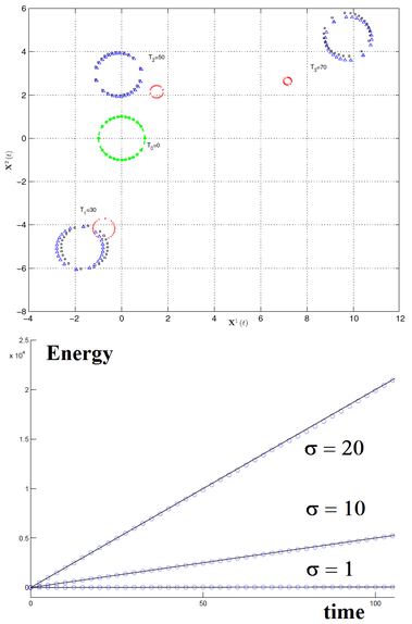
By construction, the strong LL and HOLL discretizations inherit the stability and dynamics of the linear SDEs, but it is not the case of the strong LL schemes in general. LL schemes (7.2)-(7.5) with ${\displaystyle p\leq q\leq p+2}$ are A-stable, including stiff and highly oscillatory linear equations. Moreover, for linear SDEs with random attractors, these schemes also have a random attractor that converges in probability to the exact one as the stepsize decreases and preserve the ergodicity of these equations for any stepsize. These schemes also reproduce essential dynamical properties of simple and coupled harmonic oscillators such as the linear growth of energy along the paths, the oscillatory behavior around 0, the symplectic structure of Hamiltonian oscillators, and the mean of the paths. For nonlinear SDEs with small noise (i.e., (7.1) with ${\displaystyle \mathbf {g} _{i}(t)\approx 0}$), the paths of these SLL schemes are basically the nonrandom paths of the LL scheme (4.6) for ODEs plus a small disturbance related to the small noise. In this situation, the dynamical properties of that deterministic scheme, such as the linearization preserving and the preservation of the exact solution dynamics around hyperbolic equilibrium points and periodic orbits, become relevant for the paths of the SLL scheme. For instance, Fig 4 shows the evolution of domains in the phase plane and the energy of the stochastic oscillator

${\displaystyle {\begin{array}{ll}dx(t)=y(t)dt,&x_{1}(0)=0.01\\dy(t)=-(\omega ^{2}x(t)+\epsilon x^{4}(t))dt+\sigma dw_{t},&x_{1}(0)=0.1,\end{array}}\qquad \qquad (7.6)}$

and their approximations by two numerical schemes.

Weak LL methods for SDEs

Consider the d-dimensional stochastic differential equation

${\displaystyle d\mathbf {x} (t)=\mathbf {f} (t,\mathbf {x} (t))dt+\sum \limits _{i=1}^{m}\mathbf {g} _{i}(t)d\mathbf {w} ^{i}(t),\qquad t\in \left[t_{0},T\right],\qquad \qquad (8.1)}$

with initial condition ${\displaystyle \mathbf {x} (t_{0})=\mathbf {x} _{0}}$, where the drift coefficient ${\displaystyle \mathbf {f} }$ and the diffusion coefficient ${\displaystyle \mathbf {g} _{i}}$ are differentiable functions, and ${\displaystyle \mathbf {w=(\mathbf {w} } ^{1},\ldots ,\mathbf {w} ^{m}\mathbf {)} }$ is an m-dimensional standard Wiener process.

Local Linear discretization

For a time discretization ${\displaystyle \left(t\right)_{h}}$, the order-${\displaystyle \mathbb {\beta } }$ ${\displaystyle (=1,2)}$ Weak Local Linear discretization of the solution of the SDE (8.1) is defined by the recursive relation

${\displaystyle \mathbf {z} _{n+1}=\mathbf {z} _{n}+\mathbf {\phi } _{\mathbb {\beta } }(t_{n},\mathbf {z} _{n};h_{n})+\mathbf {\eta } (t_{n},\mathbf {z} _{n};h_{n}),\quad with\quad \mathbf {z} _{0}=\mathbf {x} _{0},}$

where

${\displaystyle \mathbf {\phi } _{\mathbb {\beta } }(t_{n},\mathbf {z} _{n};\delta )=\int _{0}^{\delta }e^{\mathbf {f} _{\mathbf {x} }(t_{n},\mathbf {z} _{n})(\delta -u)}(\mathbf {f(} t_{n},\mathbf {z} _{n})+\mathbf {b} ^{\mathbb {\beta } }(t_{n},\mathbf {z} _{n})u)du}$

with

${\displaystyle \mathbf {b} ^{\mathbb {\beta } }(t_{n},\mathbf {z} _{n})={\begin{cases}\mathbf {f} _{t}(t_{n},\mathbf {z} _{n})&{\text{for }}\mathbb {\beta } =1\\\mathbf {f} _{t}(t_{n},\mathbf {z} _{n})+{\frac {1}{2}}\sum \limits _{j=1}^{m}\left(\mathbf {I} \otimes \mathbf {g} _{j}^{\intercal }\left(t_{n}\right)\right)\mathbf {f} _{\mathbf {xx} }(t_{n},\mathbf {z} _{n})\mathbf {g} _{j}\left(t_{n}\right)&{\text{for }}\mathbb {\beta } =2,\end{cases}}}$

and ${\displaystyle \mathbf {\eta } (t_{n},\mathbf {z} _{n};\delta )}$ is a zero mean stochastic process with variance matrix

${\displaystyle \mathbf {\Sigma } (t_{n},\mathbf {z} _{n};\delta )=\int \limits _{0}^{\delta }e^{\mathbf {f} _{\mathbf {x} }(t_{n},\mathbf {z} _{n})(\delta -s)}\mathbf {G} (t_{n}+s)\mathbf {G} ^{\intercal }(t_{n}+s)e^{\mathbf {f} _{\mathbf {x} }^{\intercal }(t_{n},\mathbf {z} _{n})(\delta -s)}ds.}$

Here, ${\displaystyle \mathbf {f} _{\mathbf {x} }}$, ${\displaystyle \mathbf {f} _{t}}$ denote the partial derivatives of ${\displaystyle \mathbf {f} }$ with respect to the variables ${\displaystyle \mathbf {x} }$ and t, respectively, ${\displaystyle \mathbf {f} _{\mathbf {xx} }}$ the Hessian matrix of ${\displaystyle \mathbf {f} }$ with respect to ${\displaystyle \mathbf {x} }$, and ${\displaystyle \mathbf {G} (t)=[\mathbf {g} _{1}(t),...,\mathbf {g} _{m}(t)]}$. The weak Local Linear discretization ${\displaystyle \mathbf {z} _{n+1}}$ converges with order ${\displaystyle \mathbb {\beta } }$ (=1,2) to the solution of (8.1).

Local Linearization schemes

Depending on the way of computing ${\displaystyle \mathbf {\phi } _{\mathbb {\beta } }}$ and ${\displaystyle \mathbf {\Sigma } }$ different numerical schemes could be obtained. Every numerical implementation ${\displaystyle \mathbf {y} _{n}}$ of the Weak Local Linear discretization ${\displaystyle \mathbf {z} _{n}}$ is generically called Weak Local Linearization scheme.

Order 1 WLL scheme

${\displaystyle \mathbf {y} _{n+1}=\mathbf {y} _{n}+\mathbf {B} _{14}+(\mathbf {B} _{12}\mathbf {B} _{11}^{\intercal })^{1/2}\mathbf {\xi } _{n}}$

where, for SDEs with autonomous diffusion coefficients, ${\displaystyle \mathbf {B} _{11}}$, ${\displaystyle \mathbf {B} _{12}}$ and ${\displaystyle \mathbf {B} _{14}}$ are the submatrices defined by the partitioned matrix ${\displaystyle \mathbf {B} =\mathbf {P} _{p,q}(2^{-k_{n}}{\mathcal {M}}_{n}h_{n}))^{2^{k_{n}}}}$, with

${\displaystyle {\mathcal {M}}_{n}=\left[{\begin{array}{cccc}\mathbf {f} _{\mathbf {x} }(t_{n},\mathbf {y} _{n})&\mathbf {GG} ^{\intercal }&\mathbf {f} _{t}(t_{n},\mathbf {y} _{n})&\mathbf {f} (t_{n},\mathbf {y} _{n})\\\mathbf {0} &-\mathbf {f} _{\mathbf {x} }^{\intercal }(t_{n},\mathbf {y} _{n})&\mathbf {0} &\mathbf {0} \\\mathbf {0} &\mathbf {0} &0&1\\\mathbf {0} &\mathbf {0} &0&0\end{array}}\right]\in \mathbb {R} ^{(2d+2)\times (2d+2)},}$

and ${\displaystyle \{\mathbf {\xi } _{n}\}}$ is a sequence of d-dimensional independent two-points distributed random vectors satisfying ${\displaystyle P(\xi _{n}^{k}=\pm 1)={\frac {1}{2}}}$.

Order 2 WLL scheme

${\displaystyle \mathbf {y} _{n+1}=\mathbf {y} _{n}+\mathbf {B} _{16}+(\mathbf {B} _{14}\mathbf {B} _{11}^{\intercal })^{1/2}\mathbf {\xi } _{n}}$

where ${\displaystyle \mathbf {B} _{11}}$, ${\displaystyle \mathbf {B} _{14}}$ and ${\displaystyle \mathbf {B} _{16}}$ are the submatrices defined by the partitioned matrix ${\displaystyle \mathbf {B} =\mathbf {P} _{p,q}(2^{-k_{n}}{\mathcal {M}}_{n}h_{n}))^{2^{k_{n}}}}$ with

${\displaystyle {\mathcal {M}}_{n}=\left[{\begin{array}{cccccc}\mathbf {J} &\mathbf {H} _{2}&\mathbf {H} _{1}&\mathbf {H} _{0}&\mathbf {a} _{2}&\mathbf {a} _{1}\\\mathbf {0} &-\mathbf {J} ^{\intercal }&\mathbf {I} &\mathbf {0} &\mathbf {0} &\mathbf {0} \\\mathbf {0} &\mathbf {0} &-\mathbf {J} ^{\intercal }&\mathbf {I} &\mathbf {0} &\mathbf {0} \\\mathbf {0} &\mathbf {0} &\mathbf {0} &-\mathbf {J} ^{\intercal }&\mathbf {0} &\mathbf {0} \\\mathbf {0} &\mathbf {0} &\mathbf {0} &\mathbf {0} &0&1\\\mathbf {0} &\mathbf {0} &\mathbf {0} &\mathbf {0} &0&0\end{array}}\right]\in \mathbb {R} ^{(4d+2)\times (4d+2)},}$

${\displaystyle \mathbf {J} =\mathbf {f} _{\mathbf {x} }(t_{n},\mathbf {y} _{n})\qquad \mathbf {a} _{1}=\mathbf {f} (t_{n},\mathbf {y} _{n})\qquad \mathbf {a} _{2}=\mathbf {f} _{t}(t_{n},\mathbf {y} _{n})+{\frac {1}{2}}\sum \limits _{i=1}^{m}(\mathbf {I} \otimes (\mathbf {g} ^{i}(t_{n}))^{\intercal })\mathbf {f} _{\mathbf {xx} }(t_{n},\mathbf {y} _{n})\mathbf {g} ^{i}(t_{n})}$

and

${\displaystyle \mathbf {H} _{0}=\mathbf {G} (t_{n})\mathbf {G} ^{\intercal }(t_{n})\qquad \mathbf {H} _{1}=\mathbf {G} (t_{n}){\frac {d\mathbf {G} ^{\intercal }(t_{n})}{dt}}+{\frac {d\mathbf {G} (t_{n})}{dt}}\mathbf {G} ^{\intercal }(t_{n})\qquad \mathbf {H} _{2}={\frac {d\mathbf {G} (t_{n})}{dt}}{\frac {d\mathbf {G} ^{\intercal }(t_{n})}{dt}}{\text{.}}}$

Stability and dynamics

Fig. 5 Approximate mean of the SDE (8.2) computed via Monte Carlo with 100 simulations of various schemes with h=1/16 and p=q=6.

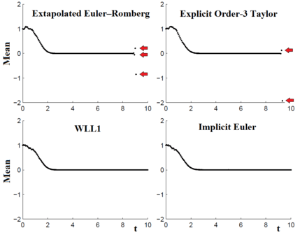
By construction, the weak LL discretizations inherit the stability and dynamics of the linear SDEs, but it is not the case of the weak LL schemes in general. WLL schemes, with ${\displaystyle p\leq q\leq p+2,}$ preserve the first two moments of the linear SDEs, and inherits the mean-square stability or instability that such solution may have. This includes, for instance, the equations of coupled harmonic oscillators driven by random force, and large systems of stiff linear SDEs that result from the method of lines for linear stochastic partial differential equations. Moreover, these WLL schemes preserve the ergodicity of the linear equations, and are geometrically ergodic for some classes of nonlinear SDEs. For nonlinear SDEs with small noise (i.e., (8.1) with ${\displaystyle \mathbf {g} _{i}(t)\approx 0}$), the solutions of these WLL schemes are basically the nonrandom paths of the LL scheme (4.6) for ODEs plus a small disturbance related to the small noise. In this situation, the dynamical properties of that deterministic scheme, such as the linearization preserving and the preservation of the exact solution dynamics around hyperbolic equilibrium points and periodic orbits, become relevant for the mean of the WLL scheme. For instance, Fig. 5 shows the approximate mean of the SDE

${\displaystyle dx=-t^{2}x{\text{ }}dt+{\frac {3}{2(t+1)}}e^{-t^{3}/3}{\text{ }}dw_{t},\qquad \qquad x(0)=1,\qquad \quad (8.2)}$

computed by various schemes.

Historical notes

Below is a time line of the main developments of the LL method.

- Pope D.A. (1963) introduces the LL discretization for ODEs and the LL scheme based on Taylor expansion. doi :10.1145/366707.367592

- Ozaki T. (1985) introduces the LL method for the integration and estimation of SDEs. The term "Local Linearization" (LL) is used for first time. doi:10.1016/S0169-7161(85)05004-0

- Biscay R. et al. (1996) reformulate the strong LL method for SDEs. doi:10.1007/BF00052324

- Shoji I. and Ozaki T. (1997) reformulate the weak LL method for SDEs. doi: 10.1111/1467-9892.00064

- Hochbruck M. et al. (1998) introduce the LL scheme for ODEs based on Krylov subspace approximation. doi:10.1137/S1064827595295337

- Jimenez J.C. (2002) introduces the LL scheme for ODEs and SDEs based on rational Padé approximation. doi:10.1016/S0893-9659(02)00041-1

- Carbonell F.M. et al. (2005) introduce the LL method for RDEs. doi: 10.1007/s10543-005-2645-9

- Jimenez J.C. et al. (2006) introduce the LL method for DDEs. doi: 10.1137/040607356

- de la Cruz H. et al. (2006, 2007) and Tokman (2006) introduce the two classes of HOLL integrators for ODEs: the integrator-based and the quadrature-based. doi:10.1007/11758501\_22, doi:10.1016/j.amc.2006.06.096 and doi:10.1016/j.jcp.2005.08.032

- de la Cruz H. et al. (2010) introduce the strong HOLL method for SDEs. doi:10.1007/s10543-010-0272-6

References

• Carbonell F.; Jimenez J.C.; Pedroso L.M. (2008). "Computing multiple integrals involving matrix exponentials,". J. Comput. Appl. Math. 213: 300–305. doi:10.1016/j.cam.2007.01.007.

• de la Cruz H.; Biscay R.J.; Carbonell F.; Jimenez J.C.; Ozaki T. (2006). "Local Linearization-Runge Kutta (LLRK) methods for solving ordinary differential equations,". Lecture Note in Computer Sciences, Springer-Verlag. Lecture Notes in Computer Science. 3991: 132–139. doi:10.1007/11758501_22. ISBN 978-3-540-34379-0.

• de la Cruz H.; Biscay R.J.; Carbonell F.; Ozaki T.; Jimenez J.C. (2007). "A higher order Local Linearization method for solving ordinary differential equations,". Appl. Math. Comput. 185: 197–212. doi:10.1016/j.amc.2006.06.096.

• de la Cruz H.; Biscay R.J.; Jimenez J.C.; Carbonell F. (2013). "Local Linearization - Runge Kutta Methods: a class of A-stable explicit integrators for dynamical systems,". Math. Comput. Modelling. 57 (3–4): 720–740. doi:10.1016/j.mcm.2012.08.011.

• de la Cruz H.; Biscay R.J.; Jimenez J.C.; Carbonell F.; Ozaki T. (2010). "High Order Local Linearization methods: an approach for constructing A-stable high order explicit schemes for stochastic differential equations with additive noise,". BIT Numer. Math. 50 (3): 509–539. doi:10.1007/s10543-010-0272-6.

• de la Cruz H.; Jimenez J.C.; Zubelli J.P. (2017). "Locally Linearized methods for the simulation of stochastic oscillators driven by random forces,". BIT Numer. Math. 57: 123–151. doi:10.1007/s10543-016-0620-2.

• M. Hochbruck.; A. Ostermann. (2011). "Exponential multistep methods of Adams-type,". BIT Numer. Math. 51 (4): 889–908. doi:10.1007/s10543-011-0332-6.

• Jimenez J.C. (2009). "Local Linearization methods for the numerical integration of ordinary differential equations: An overview,". ICTP Technical Report. 035: 357–373.

• Jimenez J.C.; Biscay R.; Mora C.; Rodriguez L.M. (2002). "Dynamic properties of the Local Linearization method for initial-value problems,". Appl. Math. Comput. 126: 63–68. doi:10.1016/S0096-3003(00)00100-4.

• Jimenez J.C.; Carbonell F. (2009). "Rate of convergence of local linearization schemes for random differential equations,". BIT Numer. Math. 49 (2): 357–373. doi:10.1007/s10543-009-0225-0.

• Jimenez J.C.; Carbonell F. (2015). "Convergence rate of weak Local Linearization schemes for stochastic differential equations with additive noise,". J. Comput. Appl. Math. 279: 106–122. doi:10.1016/j.cam.2014.10.021.

• Jimenez J.C.; de la Cruz H. (2012). "Convergence rate of strong Local Linearization schemes for stochastic differential equations with additive noise,". BIT Numer. Math. 52 (2): 357–382. doi:10.1007/s10543-011-0360-2.

• Jimenez J.C.; Pedroso L.; Carbonell F.; Hernandez V. (2006). "Local linearization method for numerical integration of delay differential equations,". SIAM J. Numer. Analysis. 44 (6): 2584–2609. doi:10.1137/040607356.

• Jimenez J.C.; Sotolongo A.; Sanchez-Bornot J.M. (2014). "Locally Linearized Runge Kutta method of Dormand and Prince,". Appl. Math. Comput. 247: 589–606. arXiv:1209.1415. doi:10.1016/j.amc.2014.09.001.

• Tokman M. (2006). "Efficient integration of large stiff systems of ODEs with exponential propagation iterative (EPI) methods,". J. Comput. Physics. 213 (2): 748–776. Bibcode:2006JCoPh.213..748T. doi:10.1016/j.jcp.2005.08.032.