Junction tree algorithm
The junction tree algorithm (also known as 'Clique Tree') is a method used in machine learning to extract marginalization in general graphs. In essence, it entails performing belief propagation on a modified graph called a junction tree. The graph is called a tree because it branches into different sections of data; nodes of variables are the branches.[1] The basic premise is to eliminate cycles by clustering them into single nodes. Multiple extensive classes of queries can be compiled at the same time into larger structures of data.[1] There are different algorithms to meet specific needs and for what needs to be calculated. Inference algorithms gather new developments in the data and calculate it based on the new information provided.[2]

Junction tree algorithm
Hugin algorithm
- If the graph is directed then moralize it to make it un-directed.
- Introduce the evidence.
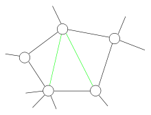
- Triangulate the graph to make it chordal.
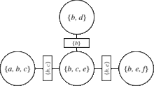
- Construct a junction tree from the triangulated graph (we will call the vertices of the junction tree "supernodes").
- Propagate the probabilities along the junction tree (via belief propagation)
Note that this last step is inefficient for graphs of large treewidth. Computing the messages to pass between supernodes involves doing exact marginalization over the variables in both supernodes. Performing this algorithm for a graph with treewidth k will thus have at least one computation which takes time exponential in k. It is a message passing algorithm.[3] The Hugin algorithm takes fewer computations to find a solution compared to Shafer-Shenoy.
Shafer-Shenoy algorithm
- Computed recursively[3]
- Multiple recursions of the Shafer-Shenoy algorithm results in Hugin algorithm[4]
- Found by the message passing equation[4]
- Separator potentials are not stored[5]
The Shafer-Shenoy algorithm is the sum product of a junction tree.[6] It is used because it runs programs and queries more efficiently than the Hugin algorithm. The algorithm makes calculations for conditionals for belief functions possible.[7] Joint distributions are needed to make local computations happen.[7]
Underlying theory

The first step concerns only Bayesian networks, and is a procedure to turn a directed graph into an undirected one. We do this because it allows for the universal applicability of the algorithm, regardless of direction.
The second step is setting variables to their observed value. This is usually needed when we want to calculate conditional probabilities, so we fix the value of the random variables we condition on. Those variables are also said to be clamped to their particular value.

The third step is to ensure that graphs are made chordal if they aren't already chordal. This is the first essential step of the algorithm. It makes use of the following theorem:[8]
Theorem: For an undirected graph, G, the following properties are equivalent:
- Graph G is triangulated.
- The clique graph of G has a junction tree.
- There is an elimination ordering for G that does not lead to any added edges.
Thus, by triangulating a graph, we make sure that the corresponding junction tree exists. A usual way to do this, is to decide an elimination order for its nodes, and then run the Variable elimination algorithm. The variable elimination algorithm states that the algorithm must be ran each time there is a different query.[1] This will result to adding more edges to the initial graph, in such a way that the output will be a chordal graph. All chordal graphs have a junction tree.[4] The next step is to construct the junction tree. To do so, we use the graph from the previous step, and form its corresponding clique graph.[9] Now the next theorem gives us a way to find a junction tree:[8]
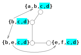
Theorem: Given a triangulated graph, weight the edges of the clique graph by their cardinality, |A∩B|, of the intersection of the adjacent cliques A and B. Then any maximum-weight spanning tree of the clique graph is a junction tree.
So, to construct a junction tree we just have to extract a maximum weight spanning tree out of the clique graph. This can be efficiently done by, for example, modifying Kruskal's algorithm. The last step is to apply belief propagation to the obtained junction tree.[10]
Usage: A junction tree graph is used to visualize the probabilities of the problem. The tree can become a binary tree to form the actual building of the tree.[11] A specific use could be found in auto encoders, which combine the graph and a passing network on a large scale automatically.[12]
Inference Algorithms

Loopy belief propagation: A different method of interpreting complex graphs. The loopy belief propagation is used when an approximate solution is needed instead of the exact solution.[13] It is an approximate inference.[3]
Cutset conditioning: Used with smaller sets of variables. Cutset conditioning allows for simpler graphs that are easier to read but are not exact.[3]
References
- Paskin, Mark. "A Short Course on Graphical Models" (PDF). Stanford.
- "The Inference Algorithm". www.dfki.de. Retrieved 2018-10-25.
- "Recap on Graphical Models" (PDF).
- "Algorithms" (PDF). Massachusetts Institute of Technology. 2014.
- Roweis, Sam (2004). "Hugin Inference Algorithm" (PDF). NYU.
- "Algorithms for Inference" (PDF). Massachusetts Institute of Technology. 2014.
- Kłopotek, Mieczysław A. (2018-06-06). "Dempsterian-Shaferian Belief Network From Data". arXiv:1806.02373 [cs.AI].
- Wainwright, Martin (31 March 2008). "Graphical models, message-passing algorithms, and variational methods: Part I" (PDF). Berkeley EECS. Retrieved 16 November 2016.
- "Clique Graph". Retrieved 16 November 2016.
- Barber, David (28 January 2014). "Probabilistic Modelling and Reasoning, The Junction Tree Algorithm" (PDF). University of Helsinki. Retrieved 16 November 2016.
- "Fault Diagnosis in an Industrial Process Using Bayesian Networks: Application of the Junction Tree Algorithm - IEEE Conference Publication". doi:10.1109/CERMA.2009.28. Cite journal requires
|journal=(help) - Jin, Wengong (Feb 2018). "Junction Tree Variational Autoencoder for Molecular Graph Generation". Cornell University. arXiv:1802.04364. Bibcode:2018arXiv180204364J.
- CERMA 2009 : proceedings : 2009 Electronics, Robotics and Automotive Mechanics Conference : 22-25 September 2009 : Cuernavaca, Morelos, Mexico. Institute of Electrical and Electronics Engineers. Los Alamitos, Calif.: IEEE Computer Society. 2009. ISBN 9780769537993. OCLC 613519385.CS1 maint: others (link)
- Lauritzen, Steffen L.; Spiegelhalter, David J. (1988). "Local Computations with Probabilities on Graphical Structures and their Application to Expert Systems". Journal of the Royal Statistical Society. Series B (Methodological). 50 (2): 157–224. doi:10.1111/j.2517-6161.1988.tb01721.x. JSTOR 2345762. MR 0964177.
- Dawid, A. P. (1992). "Applications of a general propagation algorithm for probabilistic expert systems". Statistics and Computing. 2 (1): 25–26. doi:10.1007/BF01890546.
- Huang, Cecil; Darwiche, Adnan (1996). "Inference in Belief Networks: A Procedural Guide". International Journal of Approximate Reasoning. 15 (3): 225–263. CiteSeerX 10.1.1.47.3279. doi:10.1016/S0888-613X(96)00069-2.
- Paskin, Mark A. "A Short Course on Graphical Models : 3. The Junction Tree Algorithms" (PDF). Archived from the original on March 19, 2015. Cite journal requires
|journal=(help)CS1 maint: unfit url (link) - Lepar, V., Shenoy, P. (1998). "A Comparison of Lauritzen-Spiegelhalter, Hugin, and Shenoy-Shafer Architectures for Computing Marginals of Probability Distributions." https://arxiv.org/ftp/arxiv/papers/1301/1301.7394.pdf