J curve
A J curve is any of a variety of J-shaped diagrams where a curve initially falls, then steeply rises above the starting point.
Balance of trade model
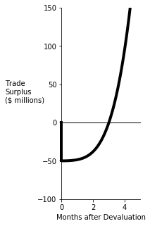
In economics, the 'J curve' is the time path of a country’s trade balance following a devaluation or depreciation of its currency, under a certain set of assumptions. A devalued currency means imports are more expensive, and on the assumption that the volumes of imports and exports change little at first, this causes a fall in the current account (a bigger deficit or smaller surplus). After some time, though, the volume of exports starts to rise because of their lower price to foreign buyers, and domestic consumers buy fewer imports, which have become more expensive for them. Eventually the trade balance moves to a smaller deficit or larger surplus compared to what it was before the devaluation.[1] Likewise, if there is a currency revaluation or appreciation the same reasoning may be applied and will lead to an inverted J curve. In Figure 1, trade starts in perfect balance, but depreciation at time 0 causes an immediate trade deficit of 50 million dollars. The balance of trade improves over time as consumers react, returning to balance at month 3 and rising to a surplus of 150 million at month 4.

Immediately following the depreciation or devaluation of the currency, the total value of imports will increase and exports remain largely unchanged due in part to pre-existing trade contracts that have to be honored. This is because in the short run, prices of imports rise due to the depreciation and also in the short run there is a lag in changing consumption of imports, therefore there is an immediate jump followed by a lag until the long run prevails and consumers stop importing as many expensive goods and along with the rise in exports cause the current account to increase (a smaller deficit or a bigger surplus).[1] Moreover, in the short run, demand for the more expensive imports (and demand for exports, which are cheaper to foreign buyers using foreign currencies) remain price inelastic. This is due to time lags in the consumer's search for acceptable, cheaper alternatives (which might not exist).
Over the longer term a depreciation in the exchange rate can usually be expected to improve the current account balance. Domestic consumers switch to domestic products and away from the now more expensive imported goods and services. Equally, many foreign consumers may switch to purchasing the products being exported into their country, which are now cheaper in the foreign currency, instead of their own domestically produced goods and services.
Empirical investigations of the J curve have sometimes focused on the effect of exchange rate changes on the trade ratio, i.e. exports divided by imports, rather than the trade balance, exports minus imports. Unlike the trade balance, the trade ratio can be logarithmically transformed regardless of whether a trade deficit or trade surplus exists.[2]
Asymmetric J-curve
The asymmetric J-curve implies that there could be an asymmetric relationship between the exchange rate changes and trade balance. The asymmetric effects of real exchange rate on trade balance were initially reported by the American economist Mohsen Bahmani-Oskooee from the University of Wisconsin–Milwaukee. However, the term asymmetric J-curve was coined by the British economists Muhammad Ali Nasir and Mary Leung. They employed cumulative dynamic multiplier analysis and reported empirical evidence of an asymmetric J-curve in an article on US trade deficit.[3]

Private equity

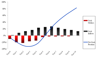
In private equity, the J curve is used to illustrate the historical tendency of private equity funds to deliver negative returns in early years and investment gains in the outlying years as the portfolios of companies mature.[4][5]
In the early years of the fund, a number of factors contribute to negative returns including management fees, investment costs and under-performing investments that are identified early and written down. Over time the fund will begin to experience unrealized gains followed eventually by events in which gains are realized (e.g., IPOs, mergers and acquisitions, leveraged recapitalizations).[6]
Historically, the J curve effect has been more pronounced in the US, where private equity firms tend to carry their investments at the lower of market value or investment cost and have been more aggressive in writing down investments than in writing up investments. As a result, the carrying value of any investment that is underperforming will be written down but the carrying value of investments that are performing well tend to be recognized only when there is some kind of event that forces the private equity firm to mark up the investment.[7]
The steeper the positive part of the J curve, the quicker cash is returned to investors. A private equity firm that can make quick returns to investors provides investors with the opportunity to reinvest that cash elsewhere. Of course, with a tightening of credit markets, private equity firms have found it harder to sell businesses they previously invested in. Proceeds to investors have reduced. J curves have flattened dramatically. This leaves investors with less cash flow to invest elsewhere, such as in other private equity firms. The implications for private equity could well be severe. Being unable to sell businesses to generate proceeds and fees means some in the industry have predicted consolidation amongst private equity firms.
Country status model

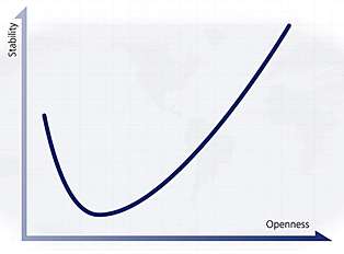
Another 'J curve' refers to the correlation between stability and openness. This theory was suggested initially by the author Ian Bremmer, in his book The J Curve: A New Way to Understand Why Nations Rise and Fall.
The x-axis of the political J curve graph measures the 'openness' of the economy in question and the y-axis measures the stability of that same state. It suggests that those states that are 'closed'/undemocratic/unfree (such as the Communist dictatorships of North Korea and Cuba) are very stable; however, as one progresses right, along the x-axis, it is evident that stability (for relatively short period of time in the lengthy life of nations) decreases, creating a dip in the graph, until beginning to pick up again as the 'openness' of a state increases; at the other end of the graph to closed states are the open states of the West, such as the United States of America or the United Kingdom. Thus, a J-shaped curve is formed.
States can travel both forward (right) and backwards (left) along this J curve, and so stability and openness are never secure. The J is steeper on the left hand side, as it is easier for a leader in a failed state to create stability by closing the country than to build a civil society and establish accountable institutions; the curve is higher on the far right than left because states that prevail in opening their societies (Eastern Europe, for example) ultimately become more stable than authoritarian regimes.
Bremmer's entire curve can shift up or down depending on economic resources available to the government in question. So Saudi Arabia's relative stability at every point along the curve rises or falls depending on the price of oil; China's curve analogously depends on the country's economic growth.
Medicine
In medicine, the 'J curve' refers to a graph in which the x-axis measures either of two treatable symptoms (blood pressure or blood cholesterol level) while the y-axis measures the chance that a patient will develop cardiovascular disease (CVD). It is well known that high blood pressure or high cholesterol levels increase a patient's risk. What is less well known is that plots of large populations against CVD mortality often take the shape of a J curve which indicates that patients with very low blood pressure and/or low cholesterol levels are also at increased risk.[8]
Political science (model of revolutions)
In political science, the 'J curve' is part of a model developed by James Chowning Davies to explain political revolutions. Davies asserts that revolutions are a subjective response to a sudden reversal in fortunes after a long period of economic growth, which is known as relative deprivation. Relative deprivation theory claims that frustrated expectations help overcome the collective action problem, which in this case may breed revolt. Frustrated expectations could result from several factors, including growing levels of inequality within a country, which may mean those who are increasingly poor relative to the rich are getting less than they expected, or a period of sustained economic development, lifting general expectations, followed by a crisis.
This model is often applied to explain social and political unrest and efforts by governments to contain this unrest. This is referred to as the Davies' J curve, because economic development followed by a depression would be modeled as an upside down and slightly skewed J.
References
- Feenstra and Taylor, Robert and Alan (2014). International Macroeconomics. New York, NY: Worth Publishers. pp. 261–264. ISBN 978-1-4292-7843-0.
- Hacker, RS and Hatemi-J, A. (2004) The effect of exchange rate changes on trade balances in the short and long run: Evidence from German trade with transitional Central European Economies. Economics of Transition. 12(4) 777-799.
- Nasir, Muhammad Ali; Mary, Leung (August 19, 2019). "US Trade Deficit, a Reality Check: New Evidence Incorporating Asymmetric and Nonlinear Effects of Exchange Rate Dynamics". Working Paper. SSRN 3439302.
- Grabenwarter, Ulrich. Exposed to the J-Curve: Understanding and Managing Private Equity Fund Investments, 2005
- A discussion on the J-Curve in private equity Archived 2013-06-12 at the Wayback Machine. AltAssets, 2006
- Understanding Private Equity Performance: The J-CURVE Effect: Earning Acceptable Returns Takes Time Archived 2008-10-27 at the Wayback Machine. California Public Employees' Retirement System
- J-Curve Effect
- Rahman, Faisal; McEvoy, John W. (August 2017). "The J-shaped Curve for Blood Pressure and Cardiovascular Disease Risk: Historical Context and Recent Updates". Current Atherosclerosis Reports. 19 (8): 34. doi:10.1007/s11883-017-0670-1. ISSN 1534-6242. PMID 28612327.