Inverse distance weighting

Inverse distance weighting (IDW) is a type of deterministic method for multivariate interpolation with a known scattered set of points. The assigned values to unknown points are calculated with a weighted average of the values available at the known points.

The name given to this type of methods was motivated by the weighted average applied, since it resorts to the inverse of the distance to each known point ("amount of proximity") when assigning weights.

Definition of the problem

The expected result is a discrete assignment of the unknown function ${\displaystyle u}$ in a study region:

${\displaystyle u(x):x\to \mathbb {R} ,\quad x\in \mathbf {D} \subset \mathbb {R} ^{n},}$

where ${\displaystyle \mathbf {D} }$ is the study region.

The set of ${\displaystyle N}$ known data points can be described as a list of tuples:

${\displaystyle [(x_{1},u_{1}),(x_{2},u_{2}),...,(x_{N},u_{N})].}$

The function is to be "smooth" (continuous and once differentiable), to be exact (${\displaystyle u(x_{i})=u_{i}}$) and to meet the user's intuitive expectations about the phenomenon under investigation. Furthermore, the function should be suitable for a computer application at a reasonable cost (nowadays, a basic implementation will probably make use of parallel resources).

Shepard's method

Historical reference

At the Harvard Laboratory for Computer Graphics and Spatial Analysis, beginning in 1965, a varied collection of scientists converged to rethink, among other things, what we now call geographic information systems.[1]

The motive force behind the Laboratory, Howard Fisher, conceived an improved computer mapping program that he called SYMAP, which, from the start, Fisher wanted to improve on the interpolation. He showed Harvard College freshmen his work on SYMAP, and many of them participated in Laboratory events. One freshman, Donald Shepard, decided to overhaul the interpolation in SYMAP, resulting in his famous article from 1968.[2]

Shepard’s algorithm was also influenced by the theoretical approach of William Warntz and others at the Lab who worked with spatial analysis. He conducted a number of experiments with the exponent of distance, deciding on something closer to the gravity model (exponent of -2). Shepard implemented not just basic inverse distance weighting, but also he allowed barriers (permeable and absolute) to interpolation.

Other research centers were working on interpolation at this time, particularly University of Kansas and their SURFACE II program. Still, the features of SYMAP were state-of-the-art, even though programmed by an undergraduate.

Basic form

Shepard's interpolation for different power parameters p, from scattered points on the surface ${\displaystyle z=\exp(-x^{2}-y^{2})}$

A general form of finding an interpolated value ${\displaystyle u}$ at a given point ${\displaystyle x}$ based on samples ${\displaystyle u_{i}=u(x_{i})}$ for ${\displaystyle i=1,2,...,N}$ using IDW is an interpolating function:

${\displaystyle u(\mathbf {x} )={\begin{cases}{\dfrac {\sum _{i=1}^{N}{w_{i}(\mathbf {x} )u_{i}}}{\sum _{i=1}^{N}{w_{i}(\mathbf {x} )}}},&{\text{if }}d(\mathbf {x} ,\mathbf {x} _{i})\neq 0{\text{ for all }}i,\\u_{i},&{\text{if }}d(\mathbf {x} ,\mathbf {x} _{i})=0{\text{ for some }}i,\end{cases}}}$

where

${\displaystyle w_{i}(\mathbf {x} )={\frac {1}{d(\mathbf {x} ,\mathbf {x} _{i})^{p}}}}$

is a simple IDW weighting function, as defined by Shepard,[2] x denotes an interpolated (arbitrary) point, x_i is an interpolating (known) point, ${\displaystyle d}$ is a given distance (metric operator) from the known point x_i to the unknown point x, N is the total number of known points used in interpolation and ${\displaystyle p}$ is a positive real number, called the power parameter.

Here weight decreases as distance increases from the interpolated points. Greater values of ${\displaystyle p}$ assign greater influence to values closest to the interpolated point, with the result turning into a mosaic of tiles (a Voronoi diagram) with nearly constant interpolated value for large values of p. For two dimensions, power parameters ${\displaystyle p\leq 2}$ cause the interpolated values to be dominated by points far away, since with a density ${\displaystyle \rho }$ of data points and neighboring points between distances ${\displaystyle r_{0}}$ to ${\displaystyle R}$, the summed weight is approximately

${\displaystyle \sum _{j}w_{j}\approx \int _{r_{0}}^{R}{\frac {2\pi r\rho \,dr}{r^{p}}}=2\pi \rho \int _{r_{0}}^{R}r^{1-p}\,dr,}$

which diverges for ${\displaystyle R\rightarrow \infty }$ and ${\displaystyle p\leq 2}$. For M dimensions, the same argument holds for ${\displaystyle p\leq M}$. For the choice of value for p, one can consider the degree of smoothing desired in the interpolation, the density and distribution of samples being interpolated, and the maximum distance over which an individual sample is allowed to influence the surrounding ones.

Shepard's method is a consequence of minimization of a functional related to a measure of deviations between tuples of interpolating points {x, u} and i tuples of interpolated points {x_i, u_i}, defined as:

${\displaystyle \phi (\mathbf {x} ,u)=\left(\sum _{i=0}^{N}{\frac {(u-u_{i})^{2}}{d(\mathbf {x} ,\mathbf {x} _{i})^{p}}}\right)^{\frac {1}{p}},}$

derived from the minimizing condition:

${\displaystyle {\frac {\partial \phi (\mathbf {x} ,u)}{\partial u}}=0.}$

The method can easily be extended to other dimensional spaces and it is in fact a generalization of Lagrange approximation into a multidimensional spaces. A modified version of the algorithm designed for trivariate interpolation was developed by Robert J. Renka and is available in Netlib as algorithm 661 in the toms library.

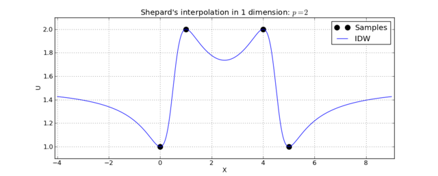
Example in 1 dimension

Shepard's interpolation in 1 dimension, from 4 scattered points and using p = 2

Łukaszyk–Karmowski metric

Yet another modification of the Shepard's method was proposed by Łukaszyk[3] also in applications to experimental mechanics. The proposed weighting function had the form

${\displaystyle w_{k}(\mathbf {x} )={\frac {1}{(D_{**}(\mathbf {x} ,\mathbf {x} _{k}))^{\frac {1}{2}}}},}$

where ${\displaystyle D_{**}(\mathbf {x} ,\mathbf {x} _{k})}$ is the Łukaszyk–Karmowski metric chosen also with regard to the statistical error probability distributions of measurement of the interpolated points.

Modified Shepard's method

Another modification of Shepard's method calculates interpolated value using only nearest neighbors within R-sphere (instead of full sample). Weights are slightly modified in this case:

${\displaystyle w_{k}(\mathbf {x} )=\left({\frac {\max(0,R-d(\mathbf {x} ,\mathbf {x} _{k}))}{Rd(\mathbf {x} ,\mathbf {x} _{k})}}\right)^{2}.}$

When combined with fast spatial search structure (like kd-tree), it becomes efficient N log N interpolation method suitable for large-scale problems.

References

1. Chrisman, Nicholas. "History of the Harvard Laboratory for Computer Graphics: a Poster Exhibit" (PDF).
2. Shepard, Donald (1968). "A two-dimensional interpolation function for irregularly-spaced data". Proceedings of the 1968 ACM National Conference. pp. 517–524. doi:10.1145/800186.810616.
3. Łukaszyk S. (2004). "A new concept of probability metric and its applications in approximation of scattered data sets". Computational Mechanics. 33 (4): 299–304. doi:10.1007/s00466-003-0532-2.

See also

• Multivariate interpolation
• Kernel density estimation