Hysteretic model

Hysteretic models are mathematical models capable of simulating the complex nonlinear behavior characterizing mechanical systems and materials used in different fields of engineering, such as aerospace, civil, and mechanical engineering. Some examples of mechanical systems and materials having a hysteretic behavior are:

• materials, such as steel, reinforced concrete, wood;
• structural elements, such as steel, reinforced concrete, or wood joints;
• devices, such as seismic isolators[1] and dampers.

Hysteretic models may have a generalized displacement ${\displaystyle u}$ as input variable and a generalized force ${\displaystyle f}$ as output variable, or vice versa. In particular, in rate-independent hysteretic models, the output variable does not depend on the rate of variation of the input one.[2][3]

Rate-independent hysteretic models can be classified into four different categories depending on the type of equation that needs to be solved to compute the output variable:

• Algebraic models
• Transcendental models
• Differential models
• Integral models

Algebraic models

In algebraic models, the output variable is computed by solving algebraic equations.

Bilinear model

Model formulation

In the bilinear model formulated by Vaiana et al. (2018),[4] the generalized force at time t, representing the output variable, is evaluated as a function of the generalized displacement as follows:

${\displaystyle f_{t}=k_{a}\left(u_{t}-u_{j}\right)+k_{b}u_{j}+s_{t}f_{0}{\text{ when }}u_{t}s_{t}<u_{j}s_{t},}$

${\displaystyle f_{t}=k_{b}u_{j}+s_{t}f_{0}{\text{ when }}u_{t}s_{t}>u_{j}s_{t},}$

where ${\displaystyle k_{a},k_{b},}$ and ${\displaystyle f_{0}}$ are the three model parameters to be calibrated from experimental or numerical tests, whereas ${\displaystyle s_{t}}$ is the sign of the generalized velocity at time ${\displaystyle t}$, that is, ${\displaystyle s_{t}=\operatorname {sign} ({\dot {u}}_{t})}$. Furthermore, ${\displaystyle u_{0}}$is an internal model parameter evaluated as:

${\displaystyle u_{0}={\frac {f_{0}}{k_{a}-k_{b}}},}$

whereas ${\displaystyle u_{j}}$ is the history variable:

${\displaystyle u_{j}={\frac {k_{a}u_{t-\Delta t}+s_{t}f_{0}-f_{t-\Delta t}}{k_{a}-k_{b}}}}$.

Hysteresis loop shapes

Figure 1.1 shows two different hysteresis loop shapes obtained by applying a sinusoidal generalized displacement having unit amplitude and frequency and simulated by adopting the Bilinear Model (BM) parameters listed in Table 1.1.

Figure 1.1. Hysteresis Loops reproduced by using the BM model parameters in Table 1.1

Table 1.1 - BM parameters

	${\displaystyle k_{a}}$	${\displaystyle k_{b}}$	${\displaystyle f_{0}}$
(a)	10.0	1.0	0.5
(b)	10.0	-1.0	0.5

Matlab code

%  =========================================================================================
%  June 2020
%  Bilinear Model Algorithm
%  Nicolò Vaiana, Research Fellow in Structural Mechanics and Dynamics, PhD 
%  Department of Structures for Engineering and Architecture 
%  University of Naples Federico II
%  via Claudio, 21 - 80124, Napoli
%  =========================================================================================

clc; clear all; close all;

%% APPLIED DISPLACEMENT TIME HISTORY

dt = 0.001;                                                                %time step
t  = 0:dt:1.50;                                                            %time interval
a0 = 1;                                                                    %applied displacement amplitude
fr = 1;                                                                    %applied displacement frequency
u  = a0*sin((2*pi*fr)*t(1:length(t)));                                     %applied displacement vector
v  = 2*pi*fr*a0*cos((2*pi*fr)*t(1:length(t)));                             %applied velocity vector
n  = length(u);                                                            %applied displacement vector length

%% 1. INITIAL SETTINGS
%1.1 Set the five model parameters
ka = 10.0;                                                                 %model parameter
kb = 1.0;                                                                  %model parameter
f0 = 0.5;                                                                  %model parameter
%1.2 Compute the internal model parameters 
u0 = f0/(ka-kb);                                                           %internal model parameter
%1.3 Initialize the generalized force vector
f  = zeros(1,n);

%% 2. CALCULATIONS AT EACH TIME STEP

for i = 2:n
%2.1 Update the history variable
uj = (ka*u(i-1)+sign(v(i))*f0-f(i-1))/(ka-kb);
%2.2 Evaluate the generalized force at time t
if (sign(v(i))*uj)-2*u0 < sign(v(i))*u(i) && sign(v(i))*u(i) < sign(v(i))*uj
    f(i) = ka*(u(i)-uj)+kb*uj+sign(v(i))*f0;
else
    f(i) = kb*u(i)+sign(v(i))*f0;
end
end

%% PLOT
figure
plot(u,f,'k','linewidth',4)
set(gca,'FontSize',28)
set(gca,'FontName','Times New Roman')
xlabel('generalized displacement'), ylabel('generalized force')
grid
zoom off

Algebraic model by Vaiana et al. (2019)

Model formulation

In the algebraic model developed by Vaiana et al. (2019),[5] the generalized force at time ${\displaystyle t}$, representing the output variable, is evaluated as a function of the generalized displacement as follows:

${\displaystyle f_{t}=\beta _{1}u_{t}^{3}+\beta _{2}u_{t}^{5}+k_{b}u_{t}+\left(k_{a}-k_{b}\right)\left[{\frac {(1+s_{t}u_{t}-s_{t}u_{j}+2u_{0})^{1-\alpha }}{s_{t}(1-\alpha )}}-{\frac {(1+2u_{0})^{1-\alpha }}{s_{t}(1-\alpha )}}\right]+s_{t}f_{0}{\text{ when }}u_{t}s_{t}<u_{j}s_{t},}$

${\displaystyle f_{t}=\beta _{1}u_{t}^{3}+\beta _{2}u_{t}^{5}+k_{b}u_{t}+s_{t}f_{0}{\text{ when }}u_{t}s_{t}>u_{j}s_{t},}$

where ${\displaystyle k_{a},k_{b},\alpha }$, ${\displaystyle \beta _{1}}$ and ${\displaystyle \beta _{2}}$ are the five model parameters to be calibrated from experimental or numerical tests, whereas ${\displaystyle s_{t}}$ is the sign of the generalized velocity at time ${\displaystyle t}$, that is, ${\displaystyle s_{t}=\operatorname {sign} ({\dot {u}}_{t})}$. Furthermore, ${\displaystyle u_{0}}$and ${\displaystyle f_{0}}$ are two internal model parameters evaluated as:

${\displaystyle u_{0}={\frac {1}{2}}\left[\left({\frac {k_{a}-k_{b}}{10^{-20}}}\right)^{1/\alpha }-1\right],}$

${\displaystyle f_{0}={\frac {k_{a}-k_{b}}{2}}\left[{\frac {\left(1+2u_{0}\right)^{1-\alpha }-1}{1-\alpha }}\right],}$

whereas ${\displaystyle u_{j}}$ is the history variable:

${\displaystyle u_{j}=u_{t-\Delta t}+s_{t}(1+2u_{0})-s_{t}\left\lbrace {\frac {s_{t}(1-\alpha )}{k_{a}-k_{b}}}\left[f_{t-\Delta t}-\beta _{1}u_{t-\Delta t}^{3}-\beta _{2}u_{t-\Delta t}^{5}-k_{b}u_{t-\Delta t}-s_{t}f_{0}+(k_{a}-k_{b}){\frac {(1+2u_{0})^{1-\alpha }}{s_{t}(1-\alpha )}}\right]\right\rbrace ^{1/(1-\alpha )}.}$

Hysteresis loop shapes

Figure 1.2 shows four different hysteresis loop shapes obtained by applying a sinusoidal generalized displacement having unit amplitude and frequency and simulated by adopting the Algebraic Model (AM) parameters listed in Table 1.2.

Figure 1.2. Hysteresis Loops reproduced by using the AM model parameters in Table 1.2

Table 1.2 - AM parameters

	${\displaystyle k_{a}}$	${\displaystyle k_{b}}$	${\displaystyle \alpha }$	${\displaystyle \beta _{1}}$	${\displaystyle \beta _{2}}$
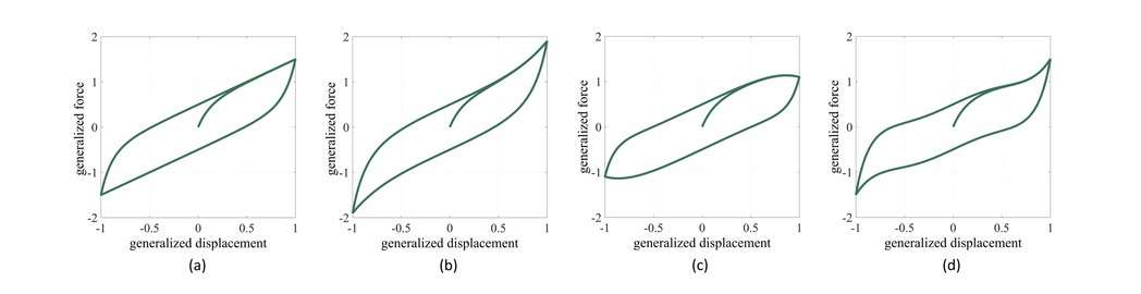
(a)	10.0	1.0	10.0	0.0	0.0
(b)	10.0	1.0	10.0	0.2	0.2
(c)	10.0	1.0	10.0	−0.2	−0.2
(d)	10.0	1.0	10.0	−1.2	1.2

Matlab code

 1 %  =========================================================================================
 2 %  September 2019
 3 %  Algebraic Model Algorithm
 4 %  Nicolò Vaiana, Post-Doctoral Researcher, PhD 
 5 %  Department of Structures for Engineering and Architecture 
 6 %  University of Naples Federico II
 7 %  via Claudio, 21 - 80125, Napoli
 8 %  =========================================================================================
 9 
10 clc; clear all; close all;
11 
12 %% APPLIED DISPLACEMENT TIME HISTORY
13 
14 dt = 0.001;                                                                %time step
15 t  = 0:dt:1.50;                                                            %time interval
16 a0 = 1;                                                                    %applied displacement amplitude
17 fr = 1;                                                                    %applied displacement frequency
18 u  = a0*sin((2*pi*fr)*t(1:length(t)));                                     %applied displacement vector
19 v  = 2*pi*fr*a0*cos((2*pi*fr)*t(1:length(t)));                             %applied velocity vector
20 n  = length(u);                                                            %applied displacement vector length
21 
22 %% 1. INITIAL SETTINGS
23 %1.1 Set the five model parameters
24 ka    = 10.0;                                                              %model parameter
25 kb    = 1.0;                                                               %model parameter
26 alfa  = 10.0;                                                              %model parameter
27 beta1 = 0.0;                                                               %model parameter
28 beta2 = 0.0;                                                               %model parameter
29 %1.2 Compute the internal model parameters 
30 u0    = (1/2)*((((ka-kb)/10^-20)^(1/alfa))-1);                             %internal model parameter
31 f0    = ((ka-kb)/2)*((((1+2*u0)^(1-alfa))-1)/(1-alfa));                    %internal model parameter
32 %1.3 Initialize the generalized force vector
33 f     = zeros(1, n);
34 
35 %% 2. CALCULATIONS AT EACH TIME STEP
36 
37 for i = 2:n
38 %2.1 Update the history variable
39 uj = u(i-1)+sign(v(i))*(1+2*u0)-sign(v(i))*((((sign(v(i))*(1-alfa))/(ka-kb))*(f(i-1)-beta1*u(i-1)^3-beta2*u(i-1)^5-kb*u(i-1)-sign(v(i))*f0+(ka-kb)*(((1+2*u0)^(1-alfa))/(sign(v(i))*(1-alfa)))))^(1/(1-alfa)));
40 %2.2 Evaluate the generalized force at time t
41 if (sign(v(i))*uj)-2*u0 < sign(v(i))*u(i) || sign(v(i))*u(i) < sign(v(i))*uj
42     f(i) = beta1*u(i)^3+beta2*u(i)^5+kb*u(i)+(ka-kb)*((((1+2*u0+sign(v(i))*(u(i)-uj))^(1-alfa))/(sign(v(i))*(1-alfa)))-(((1+2*u0)^(1-alfa))/(sign(v(i))*(1-alfa))))+sign(v(i))*f0;
43 else
44     f(i) = beta1*u(i)^3+beta2*u(i)^5+kb*u(i)+sign(v(i))*f0;
45 end
46 end
47 
48 %% PLOT
49 figure
50 plot(u, f, 'k', 'linewidth', 4)
51 set(gca, 'FontSize', 28)
52 set(gca, 'FontName', 'Times New Roman')
53 xlabel('generalized displacement'), ylabel('generalized force')
54 grid
55 zoom off

Transcendental models

In transcendental models, the output variable is computed by solving transcendental equations, namely equations involving trigonometric, inverse trigonometric, exponential, logarithmic, and/or hyperbolic functions.

Exponential models

Exponential model by Vaiana et al. (2018)

Model formulation

In the exponential model developed by Vaiana et al. (2018),[4] the generalized force at time ${\displaystyle t}$, representing the output variable, is evaluated as a function of the generalized displacement as follows:

${\displaystyle f_{t}=-2\beta u_{t}+e^{\beta u_{t}}-e^{-\beta u_{t}}+k_{b}u_{t}-s_{t}{\frac {k_{a}-k_{b}}{\alpha }}\left[e^{-\alpha (u_{t}s_{t}-u_{j}s_{t}+2u_{0})}-e^{-2\alpha u_{0}}\right]+f_{0}s_{t}{\text{ when }}u_{t}s_{t}<u_{j}s_{t},}$

${\displaystyle f_{t}=-2\beta u_{t}+e^{\beta u_{t}}-e^{-\beta u_{t}}+k_{b}u_{t}+f_{0}s_{t}{\text{ when }}u_{t}s_{t}>u_{j}s_{t},}$

where ${\displaystyle k_{a},k_{b},\alpha }$ and ${\displaystyle \beta }$ are the four model parameters to be calibrated from experimental or numerical tests, whereas ${\displaystyle s_{t}}$ is the sign of the generalized velocity at time ${\displaystyle t}$, that is, ${\displaystyle s_{t}=\operatorname {sign} ({\dot {u}}_{t})}$. Furthermore, ${\displaystyle u_{0}}$and ${\displaystyle f_{0}}$ are two internal model parameters evaluated as:

${\displaystyle u_{0}=-{\frac {1}{2\alpha }}\ln \left({\frac {10^{-20}}{k_{a}-k_{b}}}\right),}$

${\displaystyle f_{0}={\frac {k_{a}-k_{b}}{2\alpha }}\left(1-e^{-2\alpha u_{0}}\right),}$

whereas ${\displaystyle u_{j}}$ is the history variable:

${\displaystyle u_{j}=u_{t-\Delta t}+2u_{0}s_{t}+{\frac {s_{t}}{\alpha }}\ln \left[{\frac {\alpha s_{t}}{k_{a}-k_{b}}}\left(-2\beta u_{t-\Delta t}+e^{\beta u_{t-\Delta t}}-e^{-\beta u_{t-\Delta t}}+k_{b}u_{t-\Delta t}+{\frac {k_{a}-k_{b}}{\alpha }}s_{t}e^{-2\alpha u_{0}}+f_{0}s_{t}-f_{t-\Delta t}\right)\right].}$

Hysteresis loop shapes

Figure 2.1 shows four different hysteresis loop shapes obtained by applying a sinusoidal generalized displacement having unit amplitude and frequency and simulated by adopting the Exponential Model (EM) parameters listed in Table 2.1.

Figure 2.1. Hysteresis Loops reproduced by using the EM model parameters in Table 2.1.

Table 2.1 - EM parameters

	${\displaystyle k_{a}}$	${\displaystyle k_{b}}$	${\displaystyle \alpha }$	${\displaystyle \beta }$
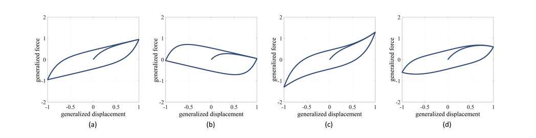
(a)	5.0	0.5	5.0	0.0
(b)	5.0	−0.5	5.0	0.0
(c)	5.0	0.5	5.0	1.0
(d)	5.0	0.5	5.0	−1.0

Matlab code

 1 %  =========================================================================================
 2 %  September 2019
 3 %  Exponential Model Algorithm
 4 %  Nicolò Vaiana, Post-Doctoral Researcher, PhD 
 5 %  Department of Structures for Engineering and Architecture 
 6 %  University of Naples Federico II
 7 %  via Claudio, 21 - 80125, Napoli
 8 %  =========================================================================================
 9 
10 clc; clear all; close all;
11 
12 %% APPLIED DISPLACEMENT TIME HISTORY
13 
14 dt = 0.001;                                                                %time step
15 t  = 0:dt:1.50;                                                            %time interval
16 a0 = 1;                                                                    %applied displacement amplitude
17 fr = 1;                                                                    %applied displacement frequency
18 u  = a0*sin((2*pi*fr)*t(1:length(t)));                                     %applied displacement vector
19 v  = 2*pi*fr*a0*cos((2*pi*fr)*t(1:length(t)));                             %applied velocity vector
20 n  = length(u);                                                            %applied displacement vector length
21 
22 %% 1. INITIAL SETTINGS
23 %1.1 Set the four model parameters
24 ka    = 5.0;                                                               %model parameter
25 kb    = 0.5;                                                               %model parameter
26 alfa  = 5.0;                                                               %model parameter
27 beta  = 1.0;                                                               %model parameter
28 %1.2 Compute the internal model parameters 
29 u0    = -(1/(2*alfa))*log(10^-20/(ka-kb));                                 %internal model parameter
30 f0    = ((ka-kb)/(2*alfa))*(1-exp(-2*alfa*u0));                            %internal model parameter
31 %1.3 Initialize the generalized force vector
32 f     = zeros(1, n);
33 
34 %% 2. CALCULATIONS AT EACH TIME STEP
35 
36 for i = 2:n
37 %2.1 Update the history variable
38 uj = u(i-1)+2*u0*sign(v(i))+sign(v(i))*(1/alfa)*log(sign(v(i))*(alfa/(ka-kb))*(-2*beta*u(i-1)+exp(beta*u(i-1))-exp(-beta*u(i-1))+kb*u(i-1)+sign(v(i))*((ka-kb)/alfa)*exp(-2*alfa*u0)+sign(v(i))*f0-f(i-1)));
39 %2.2 Evaluate the generalized force at time t
40 if (sign(v(i))*uj)-2*u0 < sign(v(i))*u(i) || sign(v(i))*u(i) < sign(v(i))*uj
41     f(i) = -2*beta*u(i)+exp(beta*u(i))-exp(-beta*u(i))+kb*u(i)-sign(v(i))*((ka-kb)/alfa)*(exp(-alfa*(sign(v(i))*(u(i)-uj)+2*u0))-exp(-2*alfa*u0))+sign(v(i))*f0;
42 else
43     f(i) = -2*beta*u(i)+exp(beta*u(i))-exp(-beta*u(i))+kb*u(i)+sign(v(i))*f0;
44 end
45 end
46 
47 %% PLOT
48 figure
49 plot(u ,f, 'k', 'linewidth', 4)
50 set(gca, 'FontSize', 28)
51 set(gca, 'FontName', 'Times New Roman')
52 xlabel('generalized displacement'), ylabel('generalized force')
53 grid
54 zoom off

Differential models

Integral models

References

1. Vaiana, Nicolò; Spizzuoco, Mariacristina; Serino, Giorgio (June 2017). "Wire rope isolators for seismically base-isolated lightweight structures: Experimental characterization and mathematical modeling". Engineering Structures. 140: 498–514. doi:10.1016/j.engstruct.2017.02.057.
2. Dimian, Mihai; Andrei, Petru (4 November 2013). Noise-driven phenomena in hysteretic systems. ISBN 9781461413745.
3. Vaiana, Nicolò; Sessa, Salvatore; Rosati, Luciano (January 2021). "A generalized class of uniaxial rate-independent models for simulating asymmetric mechanical hysteresis phenomena". Mechanical Systems and Signal Processing. 146: 106984. doi:10.1016/j.ymssp.2020.106984.
4. Vaiana, Nicolò; Sessa, Salvatore; Marmo, Francesco; Rosati, Luciano (26 April 2018). "A class of uniaxial phenomenological models for simulating hysteretic phenomena in rate-independent mechanical systems and materials". Nonlinear Dynamics. 93 (3): 1647–1669. doi:10.1007/s11071-018-4282-2.
5. Vaiana, Nicolò; Sessa, Salvatore; Marmo, Francesco; Rosati, Luciano (March 2019). "An accurate and computationally efficient uniaxial phenomenological model for steel and fiber reinforced elastomeric bearings". Composite Structures. 211: 196–212. doi:10.1016/j.compstruct.2018.12.017.