B-spline

In the mathematical subfield of numerical analysis, a B-spline or basis spline is a spline function that has minimal support with respect to a given degree, smoothness, and domain partition. Any spline function of given degree can be expressed as a linear combination of B-splines of that degree. Cardinal B-splines have knots that are equidistant from each other. B-splines can be used for curve-fitting and numerical differentiation of experimental data.

B-spline with control points/control polygon, and marked component curves

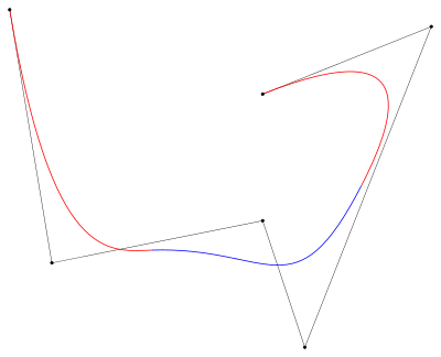
In computer-aided design and computer graphics, spline functions are constructed as linear combinations of B-splines with a set of control points.

Introduction

The term "B-spline" was coined by Isaac Jacob Schoenberg[1] and is short for basis spline.[2] A spline function of order ${\displaystyle n}$ is a piecewise polynomial function of degree ${\displaystyle n-1}$ in a variable ${\displaystyle x}$. The places where the pieces meet are known as knots. The key property of spline functions is that they and their derivatives may be continuous, depending on the multiplicities of the knots.

B-splines of order ${\displaystyle n}$ are basis functions for spline functions of the same order defined over the same knots, meaning that all possible spline functions can be built from a linear combination of B-splines, and there is only one unique combination for each spline function.[3]

Definition

Cardinal quadratic B-spline with knot vector (0, 0, 0, 1, 2, 3, 3, 3) and control points (0, 0, 1, 0, 0), and its first derivative

Cardinal cubic B-spline with knot vector (−2, −2, −2, −2, −1, 0, 1, 2, 2, 2, 2) and control points (0, 0, 0, 6, 0, 0, 0), and its first derivative

Cardinal quartic B-spline with knot vector (0, 0, 0, 0, 0, 1, 2, 3, 4, 5, 5, 5, 5, 5) and control points (0, 0, 0, 0, 1, 0, 0, 0, 0), and its first and second derivatives

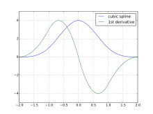
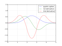
A spline of order ${\displaystyle n}$ is a piecewise polynomial function of degree ${\displaystyle n-1}$ in a variable ${\displaystyle x}$. The values of ${\displaystyle x}$ where the pieces of polynomial meet are known as knots, denoted ${\displaystyle t_{0},t_{1},t_{2},\ldots ,t_{n}}$ and sorted into non-decreasing order. When the knots are distinct, the first ${\displaystyle n-2}$ derivatives of the polynomial pieces are continuous across each knot. When ${\displaystyle r}$ knots are coincident, then only the first ${\displaystyle n-r-1}$ derivatives of the spline are continuous across that knot.

For a given sequence of knots, there is, up to a scaling factor, a unique spline ${\displaystyle B_{i,n}(x)}$ satisfying

${\displaystyle B_{i,n}(x)=\left\{{\begin{array}{ll}0&\mathrm {if} \quad x<t_{i}\quad \mathrm {or} \quad x\geq t_{i+n}\\\mathrm {nonzero} &\mathrm {otherwise} \end{array}}\right.}$

If we add the additional constraint that ${\displaystyle \sum _{i}B_{i,n}(x)=1}$ for all ${\displaystyle x}$ between the first and last knot, then the scaling factor of ${\displaystyle B_{i,n}(x)}$ becomes fixed. The resulting ${\displaystyle B_{i,n}(x)}$ spline functions are called B-splines.

Alternatively, B-splines can be defined by construction by means of the Cox–de Boor recursion formula. Given a knot sequence ${\displaystyle \ldots ,t_{0},t_{1},t_{2},\ldots }$, then the B-splines of order 1 are defined by

${\displaystyle B_{i,1}(x):=\left\{{\begin{matrix}1&\mathrm {if} \quad t_{i}\leq x<t_{i+1}\\0&\mathrm {otherwise} \end{matrix}}\right.}$

These satisfy ${\displaystyle \sum _{i}B_{i,1}(x)=1}$ for all ${\displaystyle x}$ because for any ${\displaystyle x}$ exactly one of the ${\displaystyle B_{i,1}(x)=1}$, and all the others are zero.

The higher order B-splines are defined by recursion

${\displaystyle B_{i,k+1}(x):=\omega _{i,k}(x)B_{i,k}(x)+[1-\omega _{i+1,k}(x)]B_{i+1,k}(x),}$

where

${\displaystyle \omega _{i,k}(x):={\begin{cases}{\frac {x-t_{i}}{t_{i+k}-t_{i}}},&t_{i+k}\neq t_{i}\\0,&{\text{otherwise}}\end{cases}}.}$

Properties

B-spline function is a combination of flexible bands that passes through the number of points that are called control points and creates smooth curves. These functions enable the creation and management of complex shapes and surfaces using a number of points. B-spline function and Bézier functions are applied extensively in shape optimization methods.[4]

A B-spline of order ${\displaystyle n}$ is a piecewise polynomial function of degree ${\displaystyle n-1}$ in a variable ${\displaystyle x}$. It is defined over ${\displaystyle 1+n}$ locations ${\displaystyle t_{j}}$, called knots or breakpoints, which must be in non-descending order ${\displaystyle t_{j}\leq t_{j+1}}$. The B-spline contributes only in the range between the first and last of these knots and is zero elsewhere. If each knot is separated by the same distance ${\displaystyle h}$ (where ${\displaystyle h=t_{j+1}-t_{j}}$) from its predecessor, the knot vector and the corresponding B-splines are called 'uniform' (see cardinal B-spline below).

For each finite knot interval where it is non-zero, a B-spline is a polynomial of degree ${\displaystyle n-1}$. A B-spline is a continuous function at the knots.[note 1] When all knots belonging to the B-spline are distinct, its derivatives are also continuous up to the derivative of degree ${\displaystyle n-2}$. If the knots are coincident at a given value of ${\displaystyle x}$, the continuity of derivative order is reduced by 1 for each additional coincident knot. B-splines may share a subset of their knots, but two B-splines defined over exactly the same knots are identical. In other words, a B-spline is uniquely defined by its knots.

One distinguishes internal knots and end points. Internal knots cover the ${\displaystyle x}$-domain one is interested in. Since a single B-spline already extends over ${\displaystyle 1+n}$ knots, it follows that the internal knots need to be extended with ${\displaystyle n-1}$ end points on each side, to give full support to the first and last B-spline which affect the internal knot intervals. The values of the endpoints do not matter, usually the first or last internal knot is just repeated.

The usefulness of B-splines lies in the fact that any spline function of order ${\displaystyle n}$ on a given set of knots can be expressed as a linear combination of B-splines:

${\displaystyle S_{n,\mathbf {t} }(x)=\sum _{i}\alpha _{i}B_{i,n}(x).}$

B-splines play the role of basis functions for the spline function space, hence the name. This property follows from the fact that all pieces have the same continuity properties, within their individual range of support, at the knots.[5]

Expressions for the polynomial pieces can be derived by means of the Cox–de Boor recursion formula[6]

${\displaystyle B_{i,0}(x):=\left\{{\begin{matrix}1&\mathrm {if} \quad t_{i}\leq x<t_{i+1}\\0&\mathrm {otherwise} \end{matrix}}\right.}$

${\displaystyle B_{i,k}(x):={\frac {x-t_{i}}{t_{i+k}-t_{i}}}B_{i,k-1}(x)+{\frac {t_{i+k+1}-x}{t_{i+k+1}-t_{i+1}}}B_{i+1,k-1}(x).}$[7]

That is, ${\displaystyle B_{j,0}(x)}$ is piecewise constant one or zero indicating which knot span x is in (zero if knot span j is repeated). The recursion equation is in two parts:

${\displaystyle {\frac {x-t_{i}}{t_{i+k}-t_{i}}}}$

ramps from zero to one as x goes from ${\displaystyle t_{i}}$ to ${\displaystyle t_{i+k}}$ and

${\displaystyle {\frac {t_{i+k+1}-x}{t_{i+k+1}-t_{i+1}}}}$

ramps from one to zero as x goes from ${\displaystyle t_{i+1}}$ to ${\displaystyle t_{i+k+1}}$. The corresponding Bs are zero outside those respective ranges. For example, ${\displaystyle B_{i,1}(x)}$ is a triangular function that is zero below ${\displaystyle x=t_{i}}$, ramps to one at ${\displaystyle x=t_{i+1}}$ and back to zero at and beyond ${\displaystyle x=t_{i+2}}$. However, because B-spline basis functions have local support, B-splines are typically computed by algorithms that do not need to evaluate basis functions where they are zero, such as de Boor's algorithm.

This relation leads directly to the FORTRAN-coded algorithm BSPLV which generates values of the B-splines of order n at x.[8] The following scheme illustrates how each piece of order n is a linear combination of the pieces of B-splines of order n-1 to its left.

${\displaystyle {\begin{matrix}&&0\\&0&\\0&&B_{i-2,2}\\&B_{i-1,1}&\\B_{i,0}&&B_{i-1,2}\\&B_{i,1}&\\0&&B_{i,2}\\&0&\\&&0\\\end{matrix}}}$

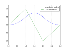
Application of the recursion formula with the knots at ${\displaystyle (0,1,2,3)}$ gives the pieces of the uniform B-spline of order 3

${\displaystyle B_{1}=x^{2}/2\qquad 0\leq x<1}$

${\displaystyle B_{2}=(-2x^{2}+6x-3)/2\qquad 1\leq x<2}$

${\displaystyle B_{3}=(3-x)^{2}/2\qquad 2\leq x<3}$

These pieces are shown in the diagram. The continuity property of a quadratic spline function and its first derivative at the internal knots are illustrated, as follows

${\displaystyle {\mbox{At }}x=1,B_{1}=B_{2}=0.5;{\frac {dB_{1}}{dx}}={\frac {dB_{2}}{dx}}=1}$

${\displaystyle {\mbox{At }}x=2,B_{2}=B_{3}=0.5;{\frac {dB_{2}}{dx}}={\frac {dB_{3}}{dx}}=-1}$

The second derivative of a B-spline of degree 2 is discontinuous at the knots:

${\displaystyle {\frac {d^{2}B_{1}}{dx^{2}}}=1,{\frac {d^{2}B_{2}}{dx^{2}}}=-2,{\frac {d^{2}B_{3}}{dx^{2}}}=-1.}$

Faster variants of the de Boor algorithm have been proposed but they suffer from comparatively lower stability.[9][10]

Cardinal B-spline

A cardinal B-spline has a constant separation, h, between knots. The cardinal B-splines for a given order n are just shifted copies of each other. They can be obtained from the simpler definition.[11]

${\displaystyle B_{i,n,t}(x)={\frac {x-t_{i}}{h}}n[0,\dots ,n](\cdot -t_{i})_{+}^{n-1}}$

The "placeholder" notation is used to indicate that the nth divided difference of the function ${\displaystyle (t-x)_{+}^{n-1}}$ of the two variables t and x is to be taken by fixing x and considering ${\displaystyle (t-x)_{+}^{n-1}}$ as a function of t alone.

A cardinal B-spline has uniform spaced knots, therefore interpolation between the knots equals convolution with a smoothing kernel.

Example, if we want to interpolate three values in between B-spline nodes (${\displaystyle {\textbf {b}}}$), we can write the signal as:

${\displaystyle {\textbf {x}}=[{\textbf {b}}_{1},0,0,{\textbf {b}}_{2},0,0,{\textbf {b}}_{3},0,0,....,{\textbf {b}}_{n},0,0]}$

Convolution of the signal ${\displaystyle {\textbf {x}}}$ with a rectangle function ${\displaystyle {\textbf {h}}=[1/3,1/3,1/3]}$ gives first order interpolated b-spline values. Second-order B-spline interpolation is convolution with a rectangle function twice ${\displaystyle {\textbf {y}}={\textbf {x}}*{\textbf {h}}*{\textbf {h}}}$, by iterative filtering with a rectangle function higher order interpolation is obtained.

Fast b-spline interpolation on a uniform sample domain can be done by iterative mean-filtering. Alternatively, a rectangle function equals Sinc in Fourier domain. Therefore, cubic spline interpolation equals multiplying the signal in Fourier domain with Sinc^4.

See Irwin–Hall distribution#Special cases for algebraic expressions for the cardinal B-splines of degree 1-4.

P-spline

The term P-spline stands for "penalized B-spline". It refers to using the B-spline representation where the coefficients are determined partly by the data to be fitted, and partly by an additional penalty function that aims to impose smoothness to avoid overfitting.[12]

Derivative expressions

The derivative of a B-spline of degree k is simply a function of B-splines of degree k-1.[13]

${\displaystyle {\frac {dB_{i,k}(x)}{dx}}=k\left({\frac {B_{i,k-1}(x)}{t_{i+k}-t_{i}}}-{\frac {B_{i+1,k-1}(x)}{t_{i+k+1}-t_{i+1}}}\right)}$

This implies that

${\displaystyle {\frac {d}{dx}}\sum _{i}\alpha _{i}B_{i,k}=\sum _{i=r-k+2}^{s-1}k{\frac {\alpha _{i}-\alpha _{i-1}}{t_{i+k}-t_{i}}}B_{i,k-1}\ on[t_{r}.t_{s}]}$

which shows that there is a simple relationship between the derivative of a spline function and the B-splines of degree one less.

Moments of univariate B-splines

Univariate B-splines, i.e. B-splines where the knot positions lie in a single dimension, can be used to represent 1-d probability density functions ${\displaystyle p(x)}$. An example is a weighted sum of ${\displaystyle i}$ B-spline basis functions of order ${\displaystyle n}$, which each are area-normalized to unity (i.e. not directly evaluated using the standard de-Boor algorithm)

${\displaystyle p(x)=\sum _{i}c_{i}\cdot B_{i,n,{\textbf {norm}}}(x)}$

and with normalization constant constraint ${\displaystyle \sum _{i}c_{i}=1}$. The k-th raw moment ${\displaystyle \mu _{k}}$ of a normalized B-spline ${\displaystyle B_{i,n,{\textbf {norm}}}}$ can be written as Carlson's Dirichlet average ${\displaystyle R_{k}}$,[14] which in turn can be solved exactly via a contour integral and an iterative sum [15] as

${\displaystyle \mu _{k}=R_{k}(\mathbf {m}$ ;\mathbf {t} )=\int _{-\infty }^{\infty }x^{k}\cdot B_{i,n,{\textbf {norm}}}(x|t_{1}\dots t_{j})dx={\frac {\Gamma (k+1)\Gamma (m)}{\Gamma (m+k)}}\cdot D_{k}(\mathbf {m} ,\mathbf {t} )}

with

${\displaystyle D_{k}={\frac {1}{k}}\sum \limits _{u=1}^{k}\left[\left(\sum \limits _{i=1}^{j}m_{i}\cdot {t_{i}}^{u}\right)D_{k-u}\right]}$

and ${\displaystyle D_{0}=1}$. Here, ${\displaystyle \mathbf {t} }$ represents a vector with the ${\displaystyle j}$ knot positions and ${\displaystyle \mathbf {m} }$ a vector with the respective knot multiplicities. One can therefore calculate any moment of a probability density function ${\displaystyle p(x)}$ represented by a sum of B-spline basis functions exactly, without resorting to numerical techniques.

Relationship to piecewise/composite Bézier

A Bézier curve is also a polynomial curve definable using a recursion from lower degree curves of the same class and encoded in terms of control points, but a key difference is that all terms in the recursion for a Bézier curve segment have the same domain of definition (usually ${\displaystyle [0,1]}$) whereas the supports of the two terms in the B-spline recursion are different (the outermost subintervals are not common). This means a Bézier curve of degree ${\displaystyle n}$ given by ${\displaystyle m\gg n}$ control points consists of about ${\displaystyle m/n}$ mostly independent segments, whereas the B-spline with the same parameters smoothly transitions from subinterval to subinterval. To get something comparable from a Bézier curve, one would need to impose a smoothness condition on transitions between segments, resulting in some manner of Bézier spline (for which many control points would be determined by the smoothness requirement).

A piecewise/composite Bézier curve is a series of Bézier curves joined with at least C0 continuity (the last point of one curve coincides with the starting point of the next curve). Depending on the application, additional smoothness requirements (such as C1 or C2 continuity) may be added.[16] C1 continuous curves have identical tangents at the breakpoint (where the two curves meet). C2 continuous curves have identical curvature at the breakpoint.[17]

To gain C2 continuity the Bézier curve loses local control, because to enforce C2 continuity the control points are dependent on each other. If a single control point moves, the whole spline needs to be re-evaluated. B-splines have both C2 continuity and local control, but they lose the interpolation property of a piecewise Bézier.[18]

Curve fitting

Usually in curve fitting, a set of data points is fitted with a curve defined by some mathematical function. For example, common types of curve fitting use a polynomial or a set of exponential functions. When there is no theoretical basis for choosing a fitting function, the curve may be fitted with a spline function composed of a sum of B-splines, using the method of least squares.[19][note 2] Thus, the objective function for least squares minimization is, for a spline function of degree k,

${\displaystyle U=\sum _{\mathrm {all} \,x}\left\{W(x)\left[y(x)-\sum _{i}\alpha _{i}B_{i,k,t}(x)\right]\right\}^{2}}$

W(x) is a weight and y(x) is the datum value at x. The coefficients ${\displaystyle \alpha _{i}}$ are the parameters to be determined. The knot values may be fixed or they too may be treated as parameters.

The main difficulty in applying this process is in determining the number of knots to use and where they should be placed. de Boor suggests various strategies to address this problem. For instance, the spacing between knots is decreased in proportion to the curvature (2nd. derivative) of the data. A few applications have been published. For instance, the use of B-splines for fitting single Lorentzian and Gaussian curves has been investigated. Optimal spline functions of degrees 3-7 inclusive, based on symmetric arrangements of 5, 6, and 7 knots, have been computed and the method was applied for smoothing and differentiation of spectroscopic curves.[20] In a comparable study, the two-dimensional version of the Savitzky-Golay filtering and the spline method produced better results than moving average or Chebyshev filtering.[21]

Computer-aided design and computer graphics

In computer-aided design and computer graphics applications, a spline curve is sometimes represented as ${\displaystyle C(t)}$, a parametric curve of some real parameter ${\displaystyle t}$. In this case the curve ${\displaystyle C(t)}$ can be treated as two or three separate coordinate functions ${\displaystyle (x(t),y(t))}$, or ${\displaystyle (x(t),y(t),z(t))}$. The coordinate functions ${\displaystyle x(t)}$, ${\displaystyle y(t)}$ and ${\displaystyle z(t)}$ are each spline functions, with a common set of knot values ${\displaystyle t_{1},t_{2},\ldots ,t_{n}}$.

Because a B-splines form basis functions, each of the coordinate functions can be expressed as a linear sum of B-splines, so we have

${\displaystyle {\begin{aligned}X(t)&=\sum _{i}x_{i}B_{i,n}(t),\\Y(t)&=\sum _{i}y_{i}B_{i,n}(t),\\Z(t)&=\sum _{i}z_{i}B_{i,n}(t).\end{aligned}}}$

The weights ${\displaystyle x_{i}}$, ${\displaystyle y_{i}}$ and ${\displaystyle z_{i}}$ can be combined to form points ${\displaystyle P_{i}=(x_{i},y_{i},z_{i})}$ in 3-d space. These points ${\displaystyle P_{i}}$ are commonly known as control points.

Working in reverse, a sequence of control points, knot values, and order of the B-spline define a parametric curve. This representation of a curve by control points has several useful properties:

1. The control points ${\displaystyle P_{i}}$ define a curve. If the control points are all transformed together in some way, such as being translated, rotated, scaled, or moved by any affine transformation, then the corresponding curve is transformed in the same way.
2. Because the B-splines are non-zero for just a finite number of knot intervals, if a single control point is moved, the corresponding change to the parametric curve is just over the parameter range of a small number knot intervals.
3. Because ${\displaystyle \sum _{i}B_{i,n}(x)=1}$, and at all times each ${\displaystyle B_{i,n}(x)\geq 0}$, then the curve remains inside the bounding box of the control points. Also, in some sense, the curve broadly follows the control points.

A less desirable feature is that the parametric curve does not interpolate the control points. Usually the curve does not pass through the control points.

NURBS

Main article: Non-uniform rational B-spline

NURBS curve – polynomial curve defined in homogeneous coordinates (blue) and its projection on plane – rational curve (red)

In computer aided design, computer aided manufacturing, and computer graphics, a powerful extension of B-splines is non-uniform rational B-splines (NURBS). NURBS are essentially B-splines in homogeneous coordinates. Like B-splines, they are defined by their order, and a knot vector, and a set of control points, but unlike simple B-splines, the control points each have a weight. When the weight is equal to 1, a NURBS is simply a B-spline and as such NURBS generalizes both B-splines and Bézier curves and surfaces, the primary difference being the weighting of the control points which makes NURBS curves "rational".

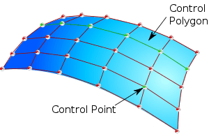
By evaluating a NURBS at various values of the parameters, the curve can be traced through space; likewise, by evaluating a NURBS surface at various values of the two parameters, the surface can be represented in Cartesian space.

Like B-splines, NURBS control points determine the shape of the curve. Each point of the curve is computed by taking a weighted sum of a number of control points. The weight of each point varies according to the governing parameter. For a curve of degree d, the influence of any control point is only nonzero in d+1 intervals (knot spans) of the parameter space. Within those intervals, the weight changes according to a polynomial function (basis functions) of degree d. At the boundaries of the intervals, the basis functions go smoothly to zero, the smoothness being determined by the degree of the polynomial.

The knot vector is a sequence of parameter values that determines where and how the control points affect the NURBS curve. The number of knots is always equal to the number of control points plus curve degree plus one. Each time the parameter value enters a new knot span, a new control point becomes active, while an old control point is discarded.

A NURBS curve takes the following form:[22]

${\displaystyle C(u)={\frac {\sum _{i=1}^{k}{N_{i,n}w_{i}P}_{i}}{\sum _{i=1}^{k}{N_{i,n}w_{i}}}}}$

Here the notation is as follows. u is the independent variable (instead of x), k is the number of control points, N is a B-spline (used instead of B), n is the polynomial degree, P is a control point and w is a weight. The denominator is a normalizing factor that evaluates to one if all weights are one.

It is customary to write this as

${\displaystyle C(u)=\sum _{i=1}^{k}R_{i,n}(u)P_{i}}$

in which the functions

${\displaystyle R_{i,n}(u)={N_{i,n}(u)w_{i} \over \sum _{j=1}^{k}N_{j,n}(u)w_{j}}}$

are known as the rational basis functions.

A NURBS surface is obtained as the tensor product of two NURBS curves, thus using two independent parameters u and v (with indices i and j respectively):[23]

${\displaystyle S(u,v)=\sum _{i=1}^{k}\sum _{j=1}^{l}R_{i,j}(u,v)P_{i,j}}$

with

${\displaystyle R_{i,j}(u,v)={\frac {N_{i,n}(u)N_{j,m}(v)w_{i,j}}{\sum _{p=1}^{k}\sum _{q=1}^{l}N_{p,n}(u)N_{q,m}(v)w_{p,q}}}}$

as rational basis functions.

See also

• Bézier curve
• Box spline
• De Boor algorithm
• I-spline
• M-spline
• Spline wavelet
• T-spline

Notes

1. Strictly speaking, B-splines are usually defined as being left-continuous.
2. de Boor gives FORTRAN routines for least-squares fitting of experimental data.

References

1. de Boor, p. 114
2. Gary D. Knott (2000), Interpolating cubic splines. Springer. p. 151
3. Hartmut., Prautzsch (2002). Bézier and B-Spline Techniques. Mathematics and Visualization. Boehm, Wolfgang., Paluszny, Marco. Berlin, Heidelberg: Springer Berlin Heidelberg. p. 63. doi:10.1007/978-3-662-04919-8. ISBN 9783662049198. OCLC 851370272.
4. Talebitooti, R.; Shojaeefard, M.H.; Yarmohammadisatri, Sadegh (2015). "Shape design optimization of cylindrical tank using b-spline curves". Computer & Fluids. 109: 100–112. doi:10.1016/j.compfluid.2014.12.004.
5. de Boor, p 113.
6. de Boor, p 131.
7. de Boor, p. 131
8. de Boor, p. 134.
9. Lee, E. T. Y. (December 1982). "A Simplified B-Spline Computation Routine". Computing. 29 (4): 365–371. doi:10.1007/BF02246763.
10. Lee, E. T. Y. (1986). "Comments on some B-spline algorithms". Computing. 36 (3): 229–238. doi:10.1007/BF02240069.
11. de Boor, p 322.
12. Eilers, P.H.C. and Marx, B.D. (1996). Flexible smoothing with B-splines and penalties (with comments and rejoinder). Statistical Science 11(2): 89-121.
13. de Boor, p. 115
14. Carlson, B.C. (1991). "B-splines, hypergeometric functions, and Dirichlet averages". Journal of Approximation Theory. 67 (3): 311–325. doi:10.1016/0021-9045(91)90006-V.
15. Glüsenkamp, T. (2018). "Probabilistic treatment of the uncertainty from the finite size of weighted Monte Carlo data". EPJ Plus. 133 (6): 218. arXiv:1712.01293. Bibcode:2018EPJP..133..218G. doi:10.1140/epjp/i2018-12042-x.)
16. Eugene V. Shikin; Alexander I. Plis (14 July 1995). Handbook on Splines for the User. CRC Press. pp. 96–. ISBN 978-0-8493-9404-1.
17. Wernecke, Josie (1993). "8". The Inventor Mentor: Programming Object-Oriented 3D Graphics with Open Inventor, Release 2 (1st ed.). Boston, MA, USA: Addison-Wesley Longman Publishing Co., Inc. ISBN 978-0201624953.
18. Zorin, Denis (2002), Bezier Curves and B-splines, Blossoming (PDF), New York University, retrieved 4 January 2015
19. de Boor, Chapter XIV, p. 235
20. Gans, Peter; Gill, J. Bernard (1984). "Smoothing and Differentiation of Spectroscopic Curves Using Spline Functions". Applied Spectroscopy. 38 (3): 370–376. Bibcode:1984ApSpe..38..370G. doi:10.1366/0003702844555511.
21. Vicsek, Maria; Neal, Sharon L.; Warner, Isiah M. (1986). "Time-Domain Filtering of Two-Dimensional Fluorescence Data". Applied Spectroscopy. 40 (4): 542–548. Bibcode:1986ApSpe..40..542V. doi:10.1366/0003702864508773.
22. Piegl and Tiller, chapter 4, sec. 2
23. Piegl and Tiller, chapter 4, sec. 4

Works cited

• Carl de Boor (1978). A Practical Guide to Splines. Springer-Verlag. ISBN 978-3-540-90356-7.
• Piegl, Les; Tiller, Wayne (1997). The NURBS Book (2nd. ed.). Springer. ISBN 978-3-540-61545-3.

Further reading

• Richard H. Bartels; John C. Beatty; Brian A. Barsky (1987). An Introduction to Splines for Use in Computer Graphics and Geometric Modeling. Morgan Kaufmann. ISBN 978-1-55860-400-1.
• Jean Gallier (1999). Curves and Surfaces in Geometric Modeling: Theory and Algorithms. Morgan Kaufmann. Chapter 6. B-Spline Curves. This book is out of print and freely available from the author.
• Hartmut Prautzsch; Wolfgang Boehm; Marco Paluszny (2002). Bézier and B-Spline Techniques. Springer Science & Business Media. ISBN 978-3-540-43761-1.
• David Salomon (2006). Curves and Surfaces for Computer Graphics. Springer. Chapter 7. B-Spline Approximation. ISBN 978-0-387-28452-1.

External links

• Weisstein, Eric W. "B-Spline". MathWorld.
• Ruf, Johannes. "B-splines of third order on a non-uniform grid" (PDF). Archived from the original (PDF) on 2013-11-06. Retrieved 2012-05-02.
• bivariate B-spline from numpy
• Interactive B-splines with JSXGraph
• TinySpline: Opensource C-library with bindings for various languages
• Uniform non rational B-Splines, Modelling curves in 2D space. Author:Stefan G. Beck
• B-Spline Editor by Shukant Pal