Build a lookup query in Excel using named ranges stored in a cell

Question

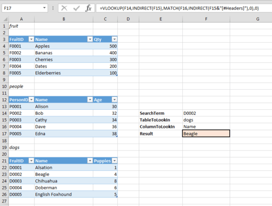
I have a spreadsheet which has a lot of named ranges, each of which is a table. I want to be able to run a lookup that will retrieve a value from any of the tables. I want to be able to store the name of the named range in a cell.

I tried:

=HLOOKUP(B14,B6,(B22+1),FALSE)

B14 was the value I wanted to look up. B6 stored the name of the named range, and using data validation can only contain the name of a named range. B22 stored the number of rows in the table and of course the +1 just stops the lookup starting in the header row.

The problem is that Excel's lookup syntax thinks that I am typing the cell range for the look-up; that B6 is the range.

I found a way to add a list of all the named ranges defined in the spreadsheet together with the range of cells using the Formulas/Defined Names/Use In Formula. I thought that I could use this as a nested lookup along the lines of

=vlookup(B6,Sheet1!$A$1,$B$77,2,FALSE) 

but although this by itself returns the correct value, it does so as if it is text. I notice that there is an = at the beginning of the string and wonder if I can detach this (MID function?), then it might be able to be recognised as a range of cells to look up. The problem with the MID function though is that you have to know the number of characters in the string and some will have more characters than others - single vs double letters for columns and units vs tens vs hundreds for rows

So I'm stuck and in need of help: any ideas would be greatly appreciated.

Answer 1

Hard to tell exactly what you're looking for without a screenshot but this might work for you. It's a dynamic VLOOKUP formula that takes table names and column names as inputs.

Here's the formula:

=VLOOKUP(F14,INDIRECT(F15),MATCH(F16,INDIRECT(F15&"[#Headers]"),0),0)

It uses INDIRECT to refer to your named ranges, and MATCH to work out which column you need to enter in your VLOOKUP.