Try this. We're going to use your PivotTable to work out which rows you don't want, then use that to create a filter column in your data table, then use our new filter column in your PivotTable.
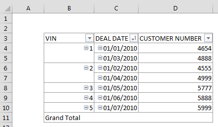
Firstly remove the subtotals from your VIN column so you get something like this:
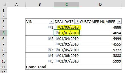
Then order your DEAL DATE column descending - so the most recent date is on top for each VIN.
Now in an adjacent column (I'm putting this in F4) enter this formula. This creates a unique identifier for the row:
=IF(B4="","",B4&"-"&C4&"-"&D4)
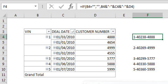
The IF() ignores all the old deals, and for recent deals we create our concatenated identifier, composed of VIN, DEAL DATE and CUSTOMER NUMBER.
Now go to your main data table. Add a new column and concatenate the columns for VIN, DEAL DATE and CUSTOMER NUMBER (in the same way we did in our formula above).
Add another column to your data table which we'll use as a filter. Enter this formula (change the worksheet name to wherever your Pivot Table is):
=IF(ISERROR(IF(MATCH(F2,YourPivotTableWorksheet!F:F,0),"Recent Deal")),"Old Deal",IF(MATCH(F2,YourPivotTableWorksheet!F:F,0),"Recent Deal"))

Adjust your PivotTable range to add in these 2 new columns, and use your new filter column to exclude the rows you don't need.
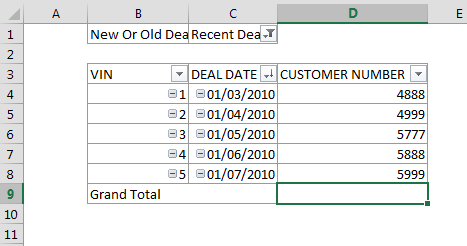


What have you tried? Can you post an image (with anonymised data of course) to imgur.com and paste the link? – Andi Mohr – 2015-10-12T15:37:38.200
@AndiMohr I've tried adding a calculated item but I'm getting an error "References to multiple item names per field cannot be included in PivotTable formulas". I edited my post to include an image. – Alexander John – 2015-10-12T15:51:16.563