Sum values in specific rows based on whether the row has a value that belongs to a range

Question

Here's what I'm trying to do: I have a table that has several metrics (example: revenue, cost, etc.) for about a hundred different accounts. I can't modify this sheet because it gets auto-updated by a different group.

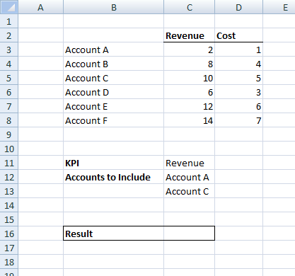
On a summary page, I want to be able to pick a metric, say revenue (Cell C11), and specify a set of accounts (Named Range C12:C13). The result (Cell C16) should be the sum of the revenues of all the specified accounts.

For just one account, I had:

=SUM(IF(B3:B8=SelectedAccount, IF(C2:D2=SelectedMetric, C3:D8)))

But I want to be able to do this for multiple accounts. The list of accounts is variable, and is around 30 accounts, so can't just do chain together a couple of the above formula.

Here's the simplified example, in image format. (Result should be 12).

Any help would be greatly appreciated!

Answer 1

=SUM(INDEX(C2:D7,0,MATCH(SelectedMetric,MetricHeaders,0))*IFERROR(MATCH(AccountNames,SelectedAccount,0)>0,0))

Where:

• MATCH(SelectedMetric,MetricHeaders,0)) - looks for the column number of the selected metric
• INDEX(C2:D7,0,MATCH(...)) - select the desired column from the table
• MATCH(AccountNames,SelectedAccount,0)>0 - selects rows which are in the selected accounts
• IFERROR(MATCH(...)>0,0) - converts errors to 0

Similarly to the formula in the original question, this is also an array formula, need to be entered by CTRL + SHIFT + ENTER