Creating a table similar to pivot table

Question

I'm not sure how to explain it, but I hope this example makes it clear.

Data:

Yes/No | Place1 | Place2 | Place3
----------------------------------
Yes    | Thing1 | Thing2 | Apple
No     | Apple  | Thing2 | Thing1
Yes    | Orange | Banana | Apple

Desired output:

        | Place1 | Place2 | Place3
 ----------------------------------
 Thing1 |  100%  |        |   0%
 Thing2 |        |   50%  |        
 Apple  |   0%   |        |  100%
 Orange |  100%  |        |
 Banana |        |  100%  |       

The percentages correspond to the percentage of Yes for that place thing combo. So the 50% there for Thing2xPlace2 is because in the data, 1 out of 2 times that Thing2 was in Place2, the corresponding Yes/no column was yes.

I think I can get it working for fixed values for things, but I would like that to be more dynamic. If there is a new value in the data, there should be a new row in the table.

Any tips are much appreciated, and thanks in advance!

Edit: preferably for google spreadsheets but if there's a way in excel i might be able to do the same in google docs

Answer 1

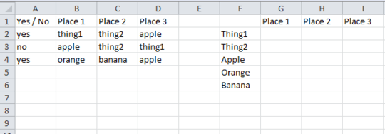
I setup a sheet as you did above

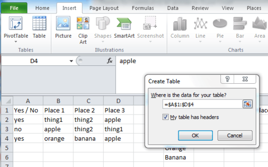
I then converted the data part to a table with headers

I then used a COUNTIFS formula in cell G2 to count the number of "yes" and matched it to F2 and Place 1 in the table.

That result is then divided by the number of "yes" and "No" that Match cell F2 for Place 1 in the table using the same COUNTIFS format in the table to get the percentage.

The IFERROR at the beginning gets rid of #DIV/0 errors.

Here is the complete formula for G2

=IFERROR(COUNTIFS(Table3[[Place 1 ]],F2,Table3[Yes / No],"yes") / (COUNTIFS(Table3[[Place 1 ]],F2,Table3[Yes / No],"yes")+COUNTIFS(Table3[[Place 1 ]],F2,Table3[Yes / No],"no")),"")

I then drag filled the formula down for each item in Column G.

I then created the same formula with appropriate references for Place 2 and Place 3 and filled down for each

If you add rows to the table it will automatically update the values on the right because you referenced the columns in the table.