Excel Vlookup for 2nd, 3rd, 4th or 5th text value, instead of 1st matching value

I have rows of possible duplicate employee ID #'s, with another column of different values for the same person. I need a single column of unique ID's with the certifications transposed in the same row. For example:

ID       Certification
0123     CPR
456      CPR
456      Nursing
456      Safety
789      Engineering
966      CPR
966      Safety

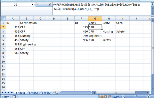
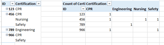
So for ID 0123 they only have one, there would only be one value to retrieve, but for ID 456, I would need the Excel sheet to have the Certification values in the same row for the ID but across as many times as the number of certifications there are:

ID    Certif1        Certif2
456    CPR           Safety

Any ideas would be appreciated as the values are all text. I also am using Excel 10.

Kelly

Posted 2014-08-18T20:34:42.777

Reputation: 13

possible duplicate of Excel 2007 transpose/combine multiple rows into one and How to combine values from multiple rows into a single row in Excel?; see also Excel 2010 Move data from multiple columns/rows to a single row and maybe others.

– G-Man Says 'Reinstate Monica' – 2014-08-18T21:02:37.603

I'm confused - why does your output row for 456 not have a column for Nursing? – Mike Honey – 2014-08-19T03:34:20.003

It should have nursing, an oversight on my part. K – Kelly – 2014-08-19T13:53:47.117

Answers

You can build the transformed table in two steps.

Step 1: Generate list of unique IDs.

You can do this with the Advanced Filter tool. Select the column of IDs including the header and click Advanced Filter on the Data ribbon. Check the Unique Records Only checkbox, and choose to Copy to another location. Set the location for the output to go to and click OK. This will give you the list of unique IDs for the rows of your new table.

Step 2: Get certifications that match each ID in new columns.

You can use an array formula to return the matching certifications to the appropriate columns. In the row of the first record in your new table, enter the formula below, adjusted to match your sheet.

=IFERROR(INDEX($B$1:$B$8,SMALL(IF($A$1:$A$8=$F2,ROW($B$1:$B$8),1000000),COLUMN()-6)),"")

where A1:B8 is the original data you provided,
F2 is the ID in the new table you are looking for certifications for, and
COLUMN()-6 equals 1 for the Certif1 column, 2 for Certif2 column (you'll have to adjust the subtraction term to match your data).

Once entered, select the cell, click inside the formula bar and press Ctrl+Shift+Enter. This will enter the formula as an array formula.

After doing this, fill the formula down the column. Then fill it over to as many columns as you need (just 3 for your sample data since 456 has 3 certifications). That should give you what you want.

Sample:

enter image description here

Excellll

Posted 2014-08-18T20:34:42.777

Reputation: 11 857

1Using COLUMNS($A:A) instead of COLUMN()-6 in the first cell means that no manual adjustment is required, wherever the OP decides to place that formula. The same applies to ROWS($1:1) in place of constructions with ROW(). – XOR LX – 2014-08-19T06:59:03.270

This formula worked, thank you so much!!!! ;-) – Kelly – 2014-08-19T13:21:46.897

You could use a pivot table to build a tabular structure, though slightly different from the layout you describe.

enter image description here

For the example on the left, drag ID and Certification into the row area and select a tabular layout. Remove any totals and sub totals.

For the example on the left, drag ID to the row and Certification to the column area and Certification again to the Values area.

teylyn

Posted 2014-08-18T20:34:42.777

Reputation: 19 551

I'm trying to avoid listing each certification in columns for every employee as not all employees have these. I've been modifying my pivot table to try options but not getting the result I'm looking for. Thanks. – Kelly – 2014-08-19T13:05:05.277