0
2
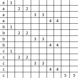
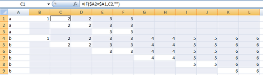
So frustrating! I get data sent to me and it looks like this:
a  1
a     2  2
a           3  3
b  1
b     2  2
b           3  3
b                 4  4
b                       5  5
b                             6  6
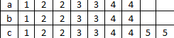
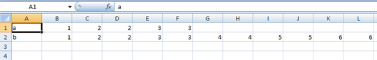
and I need it to look like this:
a  1  2  2  3  3
b  1  2  2  3  3  4  4  5  5  6  6
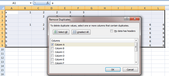
I have about 30 columns that need to move to the top value in their group, then removing the duplicates (to which there are about 33 rows of duplicates, trying to get it down to about 8 rows). I have been searching forums for several days and trying bits and pieces of code. I am having such a tough time with VBA!!!!
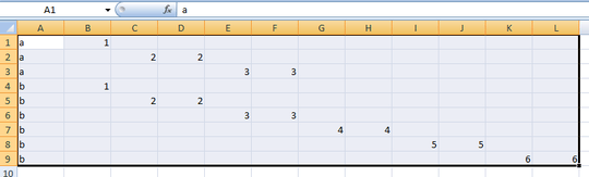
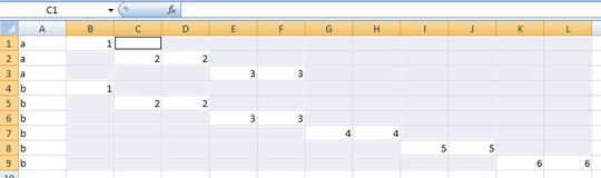
Same illustration, but graphically:
 →
→ 

frustrated529
Posted 2014-05-29T15:16:12.730
Reputation: 11

30 columns? Maybe I'm missing something, but this seems like a manual operation that'll take no more than 5-10 minutes. – Wutnaut – 2014-05-29T15:23:48.800
Your question is confusing. Your title says "Move data from multiple columns to a single row". But the example you provide (a1a22a33...->a12233...) looks like sorting a row (and possibly eliminating duplicates). Can you be more specific about exactly what you want to do? – mkasberg – 2014-05-29T15:25:50.513
Sorry, I just edited it to make it more visually correct. I just need to move all the values in the columns 'up' to the first value that starts the duplicates in the primary column. – frustrated529 – 2014-05-29T15:26:43.663
1Am I understanding you correctly; you are trying to remove the
---so you can remove duplicates and sort the data? – CharlieRB – 2014-05-29T16:04:10.767Is the identifier (a or b in the examples) always a single character? Is there any consistency to the offsets between rows of data, for instance you've got a space after the b on the line with two 3s? – Jason Aller – 2014-05-29T16:07:02.710
Good question. I am not allowed to post images yet so the '----' are supposed to be blank columns. So, this might be confusing, each character is supposed to signify a different column. Letter "A and B" column A/row1, Number 1 = Column B/row1, first '2' = column C/row2, second '2' = Column D/row2, first '3' = Column E/row 3, second '3' = Column F/row 3, first '4' = Column G/row 4, etc to the last '6' = column L/row 6 – frustrated529 – 2014-05-29T16:11:16.287
Can you upload a picture to hostr.co or similar and link it? Struggling to understand the problem.
– Jonny Wright – 2014-05-29T16:16:36.390Jason, the identifier is not a single character, they are names – frustrated529 – 2014-05-29T16:17:31.920
http://hostr.co/CBfMGH4BdNDF – frustrated529 – 2014-05-29T16:27:14.693
Do the names (represented by a and b in your example) have a fixed width? Do additional rows always only include new information after the length of the previous row, or could there be "a 1 - 3" followed by "a - 2" such that the output is supposed to be "a 1 2 3". Is the supplied data in order, like the example? – Jason Aller – 2014-05-29T16:27:14.940
No, they do not have a fixed width. – frustrated529 – 2014-05-29T16:29:15.340
Excellll,I will try the below answer. If it works, do you think I can record a MACRO to accomplish the steps? – frustrated529 – 2014-05-29T16:41:26.047