0
I have data that has dates, returns, and two columns of dummy variables. I would like to know how to use a formula to only show data when the dummy variable indicates a hit. My data looks like this:
    date      Return    A   B
    1/1/2014    0.18    0   0
    1/2/2014    0.97    0   1
    1/3/2014    0.73    0   0
    1/4/2014    0.85    1   0
    1/5/2014    0.19    1   0
    1/6/2014    0.80    0   0
    1/7/2014    0.50    0   0
    1/8/2014    0.27    0   0
    1/9/2014    0.94    0   0
    1/10/2014   0.40    0   0
    1/11/2014   0.56    0   0
    1/12/2014   0.40    1   0
    1/13/2014   0.40    1   0
    1/14/2014   0.43    1   1
    1/15/2014   0.44    0   1
    1/16/2014   0.90    0   0
    1/17/2014   0.35    0   0
And I would like it to output two tables:
    DUMMY A TABLE
    date    Return  A   B
    1/4/2014    0.85    1   0
    1/5/2014    0.19    1   0
    1/12/2014   0.40    1   0
    1/13/2014   0.40    1   0
    1/14/2014   0.43    1   1
and
    DUMMY B TABLE
    date    Return  A   B
    1/2/2014    0.97    0   1
    1/14/2014   0.43    1   1
    1/15/2014   0.44    0   1
I have figured how to do it using sort copy / paste, but I would like a formula to make it a more efficient template

user3537689
Posted 2014-04-15T21:30:51.050
Reputation: 3

Unfortunately, no as it is not scaleable. In the workbooks I am working with, I have 6-9 dummy variables that I have to run fairly often with different data. I am currently copy/pasting, but if I could code it, I could save a ton of time. – user3537689 – 2014-04-15T21:50:26.850
Each time I run the report, the number of indicators in each columns change. Would a macro be able to only pull the ones that are equal to 1 when that number of indicators changes each time? – user3537689 – 2014-04-15T21:56:50.420
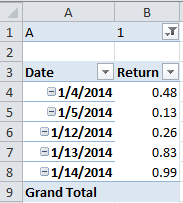
Have you tried pivot tables? – Madball73 – 2014-04-16T12:11:51.733
What do you mean? Pivot it 90 degrees? – user3537689 – 2014-04-16T15:10:01.293
I'll take that as a no :) There is an excel function called pivot tables (use Excel help to learn how to use). It allows you to create filterable tables over other tables (and accumulate data, but this is not one of your needs). I'll add as answer. – Madball73 – 2014-04-16T16:04:34.947