Excel combine rows dollar amount with matching row values?

1

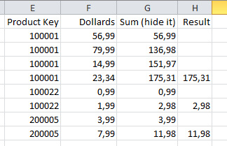
I've ran into a problem with Excel, I have the below table

enter image description here

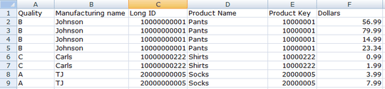
Basically, I'm trying to figure out how to make all rows that have the same product key combine, except calculating the dollar amount for each matching row for that new row. For example, rows 8 and 9 would match on row E, and then add 3.99 and 7.99. The result would be only one row with all the same information except for Dollars which would be 11.98.

Can anyone help me figure out how to go about doing this?

ben

Posted 2014-03-25T14:18:02.423

Reputation: 11

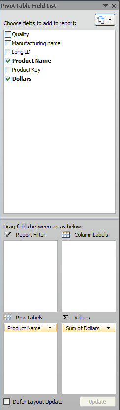
2Did you try using Pivot tables? – Dave – 2014-03-25T14:45:51.503

1A problem directly addressed by Pivot Table, as @DaveRook mentioned – Raystafarian – 2014-03-25T15:02:12.180

Answers

3

Sounds like a job for pivot table!

Highlight your table and go to Insert → pivot table and arrange it how you want. I'd do the following -

enter image description here

Raystafarian

Posted 2014-03-25T14:18:02.423

Reputation: 20 384

What a wonderfully clear answer... – Dave – 2014-03-25T21:42:08.587

1

In my opinion, the pivot table/report is the way to go. But if you would rather have the results below the table, you can use the SUMIFS function to total the dollars which meets the product key criteria in the range you specify. You can use multiple criteria if needed.

SUMIFS(sum_range, criteria_range1, criteria1, [criteria_range2, criteria2], …)

Below I used the example to build subtotals below the table.

enter image description here

Here it is again with the formula highlights.

enter image description here

CharlieRB

Posted 2014-03-25T14:18:02.423

Reputation: 21 303

0

Without Pivot table, to get your result (as far I understand your need) :

Result

Enter thoses formulas :

in G row: =IF(E2=C1;E1;0)+F2

in H row: =IF(E2=E3;"";G2)

(then you could hide the G row)

CmPi

Posted 2014-03-25T14:18:02.423

Reputation: 166