Manually populate a Pivot Table

Question

This is really a stupid question because I am supposed to know the answer.

I have a data file that looks like this:

Tech    ||  Workdate   || Fail || Manual
Joe     || 2013-05-23  ||   6  ||   1
Joe     || 2013-05-24  ||   2  ||   1
Tom     || 2013-05-23  ||   0  ||   2
Tom     || 2013-05-24  ||   2  ||   0

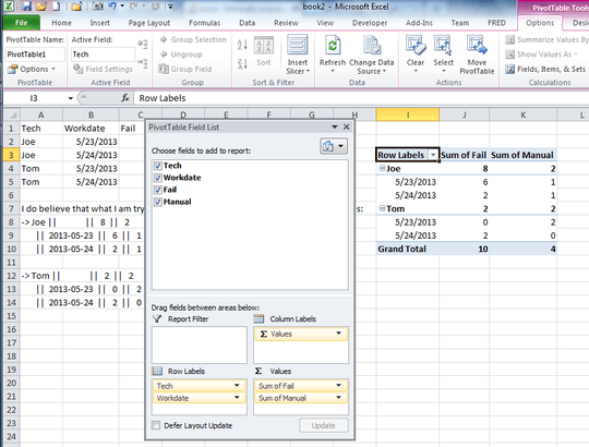
I do believe that what I am trying to accomplish is obvious, except to me. Here it is:

-> Joe ||              ||   8  ||   2
       ||  2013-05-23  ||   6  ||   1
       ||  2013-05-24  ||   2  ||   1

-> Tom ||              ||   2  ||   2
       ||  2013-05-23  ||   0  ||   2
       ||  2013-05-24  ||   2  ||   0

The pivot table wizard will only accept math functions such as count in the data field. I don't want the count of the 'fail' and 'Manual'. That's always going to be 1 for both. I need the actual values with a summation under each tech's name. Where am I going wrong?

Here's some helpful details: Macbook Pro, OS 10.8.3 Excel Mac, v2011, 14.1.3

Answer 1

The following Pivot Table setting should produce what you are looking for:

Answer 2

You should be able to click on the item in the Values section, choose "Value Field Settings," and then change from Count to Sum.